Introduction to Sorting
Sorting is one of the most important problems that is studied in computer science. It is necessary for any application to run smoothly.
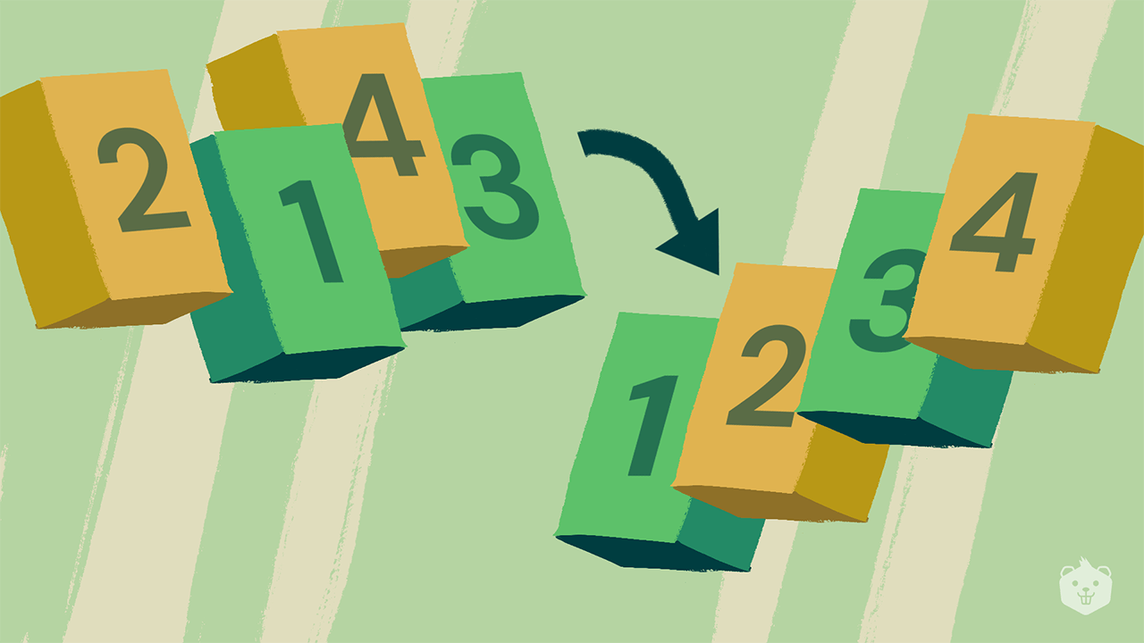
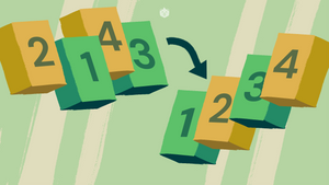
Say you just started a clothing website, and you need to add a filter that sorts the clothes according to their price.
You definitely need code that will sort these clothes in a particular order.
There are some inbuilt sorting functions in most programming languages, that will easily help you do this.
But in the 1950s, computer scientists had just begun to invent sorting algorithms.
Hoare invented Quick Sort in 1961. Before you start reading about Quick Sort, think about how you would create a sorting algorithm. Doing this will make you appreciate how well thought out Quick Sort is.
Sorting particular items would mean arranging them in a particular order. For the items to be orderable, each item must be comparable with every other item. So the basic operation you’d need to perform to sort a list of items would be comparisons. Now the question is, how would you perform these comparisons. Comparing each and every item in a list with every other item is tedious.
For example, you can sort the letters of a word in alphabetical order. But you can’t sort a list of different colors, unless some sorting criteria is specified.
But a list can have identical elements, it can be empty, it can have just one element, or all the elements can be identical. Most sorting algorithms take care of all of these cases.
Quick Sort offers a solution of its own for sorting a list of items in an efficient way.
In this blog, you will learn two variants of Quick Sort
- Quick Sort with the first element in the array as the pivot
- Quick Sort with a random pivot
What is Quick Sort
Quick Sort is a Divide and Conquer algorithm.
Divide and conquer is a problem-solving technique where a problem is divided recursively into smaller instances. The solutions of these instances are then combined, which gives the solution for the original problem itself.
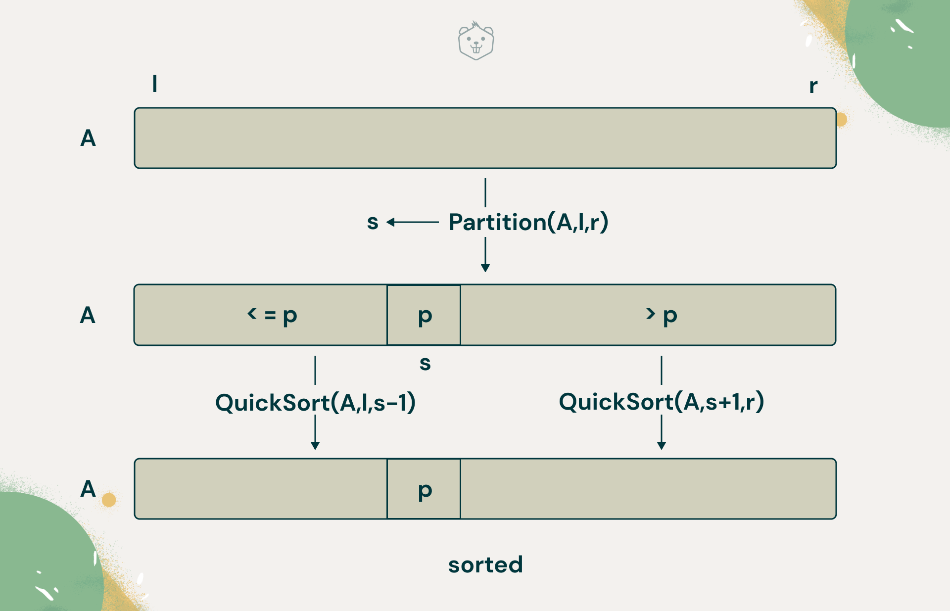
Quick Sort will rearrange the elements in a given array that needs to be sorted, such that it achieves a partition. An element ‘s’ is placed in this position of partition in the array, such that all the elements to the left of s are smaller than s and all the elements to the right of s are larger than s.
The element ‘s’ will be in its final position in the array once a partition has been found. Quick Sort will now proceed to recursively sort the left and right subarrays.
Check out this other Divide and Conquer algorithm in detail:

Algorithm Design for Quick Sort with the first element as the pivot
Pseudocode
QuickSort(A[l..r])
//Input:A subarray A[l..r] of A[0..n-1], where l and r are left most and
//right most indices of the subarray of A
//Output: Subarray A[l..r] sorted in non decreasing order

If l < r

	s = Partition(A[l..r])

   	 //s is split position returned by partition subroutine
	//Apply Quick Sort to array elements to the left of the partition s
    QuickSort(A,l,s-1)

	//Apply Quick Sort to array elements to the right of the partition s
    QuickSort(A,s+1,r)
You can see that there are two subroutines, Partition and Quick Sort. First, you need to find a pivot(s).
What is Pivot in sorting
It is an element that needs to be placed at a position at which the array can be partitioned such that all elements to the left of the pivot are at most equal to the pivot, and all elements to the right of the pivot are greater than the pivot.
Partition will find a position or index ‘s’ where the pivot can be placed and returns this. The array now has now been split, based on this partition. The split index is then passed to QuickSort, a recursive function, which will sort the left subarray first, and then proceed to sort the right subarray, using the same idea.
Understand this better with the illustration below:
In this algorithm, you will take the first element as the pivot, and use Partition to find a split position for it. But wait, what about sorting? Partition implements this as well. Let's look at how Partition works now.
Partition(A[l..r])
//Partitions a subarray by using its first element as pivot.
//Input: A subarray A[l..r] of A[0..n-1] defined by its left and right
//indices l and r, l < r
//Output: A partition of A[l..r], with the split position returned as the //function’s value

//Assign the first element as pivot
p = A [ l ]
i = l; j = r + 1
repeat
//Traverse  left to right with i , until you find an element greater than or //equal to p
repeat i = i + 1 until A[i] >= p
//Traverse right to left with j , until you find an element lesser than or //equal to p
repeat j = j - 1 until A[j] <= p
swap(A[ i ], A[ j ])
//repeat the above steps until i crosses j
until i >= j

swap(A[ i ],  A[ j ] ) //Undo the last swap when i >  j
swap(A[ l ],  A[ j ] )
return j
i: Starts from the leftmost index of the array. Scans left to right, comparing each element to pivot. Skips over elements that are lesser than the pivot. So, keep incrementing i, until you find a value greater than or equal to the pivot.
j: Starts from the rightmost index of the array. Scans right to left, comparing each element to the pivot. Skips over elements that are greater than the pivot. So keep decrementing j, until you find a value lesser than or equal to the pivot.
Now think about what has been accomplished, if you can't increment i anymore, and decrement j anymore. They’ve halted. Where have they halted?
There are three scenarios that might occur:
- i has not crossed j, i < j
- i has crossed j, i > j
- i and j are at the same position, i = j
Case 1: i < j
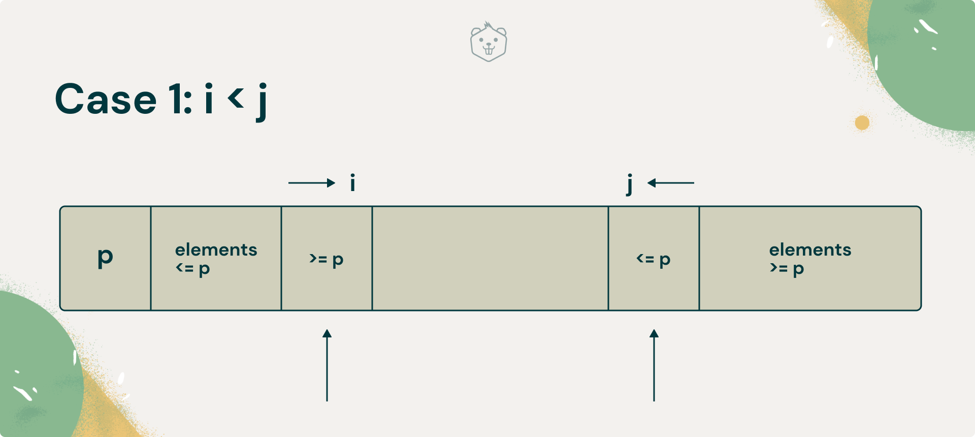
If i < j, and they’ve halted, it must mean that i has found an element that must be placed to the right of the pivot, and j has found an element that must be placed to the left of the pivot.
So swap them and resume the scans. Keep in mind that you have not found the position where you need to place the pivot yet.
Case 2: i > j
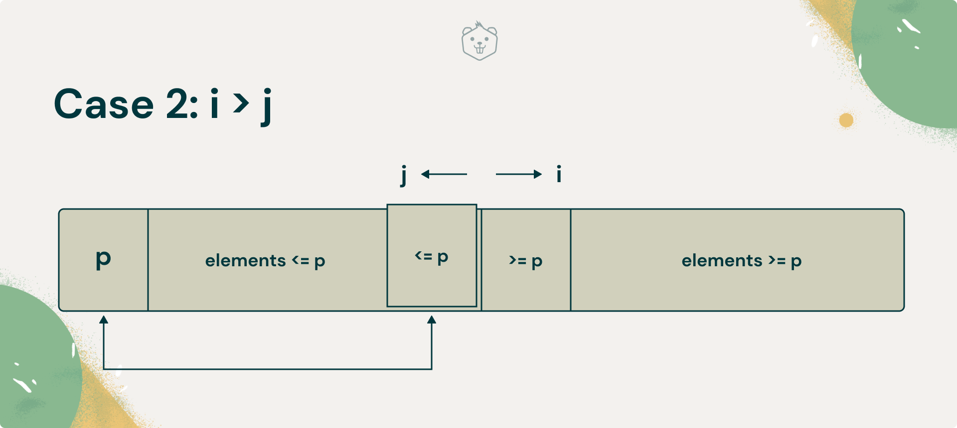
In this case, you must pay attention to what value j has. In the last swap, you would have swapped two elements, the element at j, will be greater than the one at i.
What you must do now is undo this swap. Brainstorm why you need to do this.
If you don’t undo this swap, an element greater than the pivot will lie to the left of the pivot, and an element lesser than the pivot to its right.
Once you undo this swap, you will have an element at j that is smaller than the pivot. Now swap A [ l ](which is the pivot) and A [ j ].
Case 3: i = j
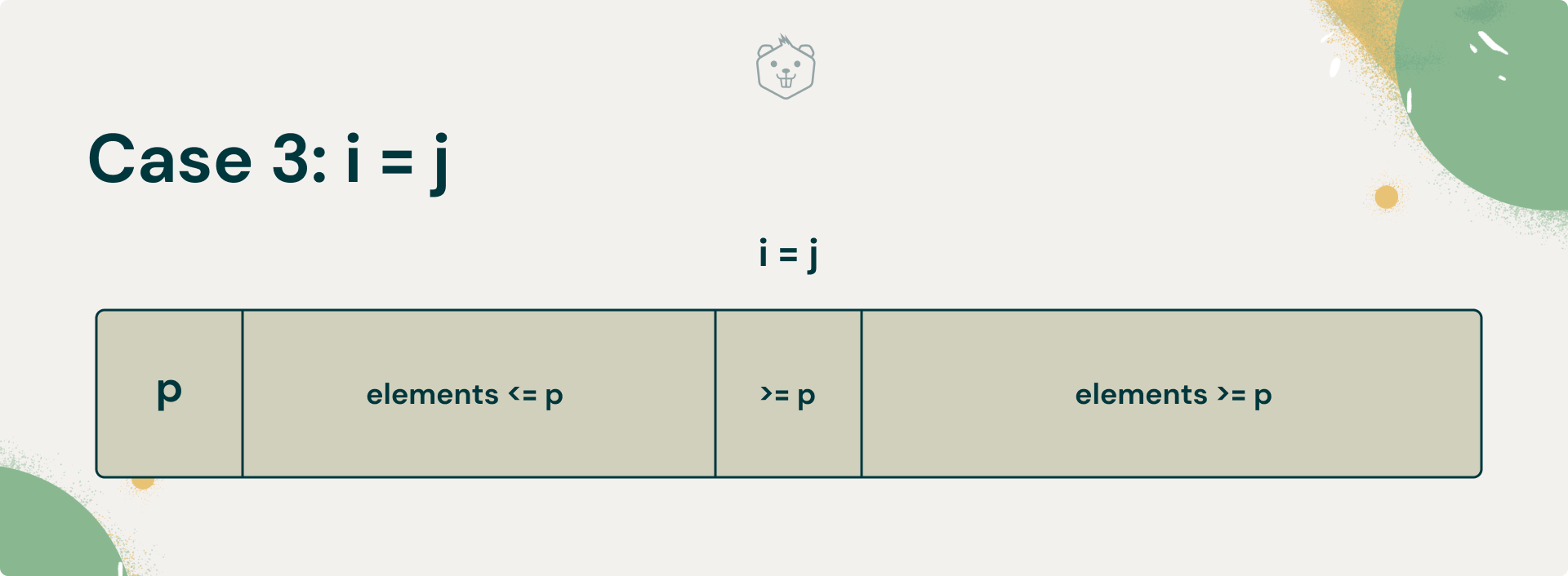
Finally, if the scanning indices have stopped pointing to the same indices, the value they are pointing to must be equal to ‘s’, the index of partition. The pivot is placed here.
Therefore, the array is partitioned with split position i = j = s .
In the next section, you will visualize Quick Sort with an example, and learn about how Quick Sort uses recursion.
Visualizing Quick Sort with an example
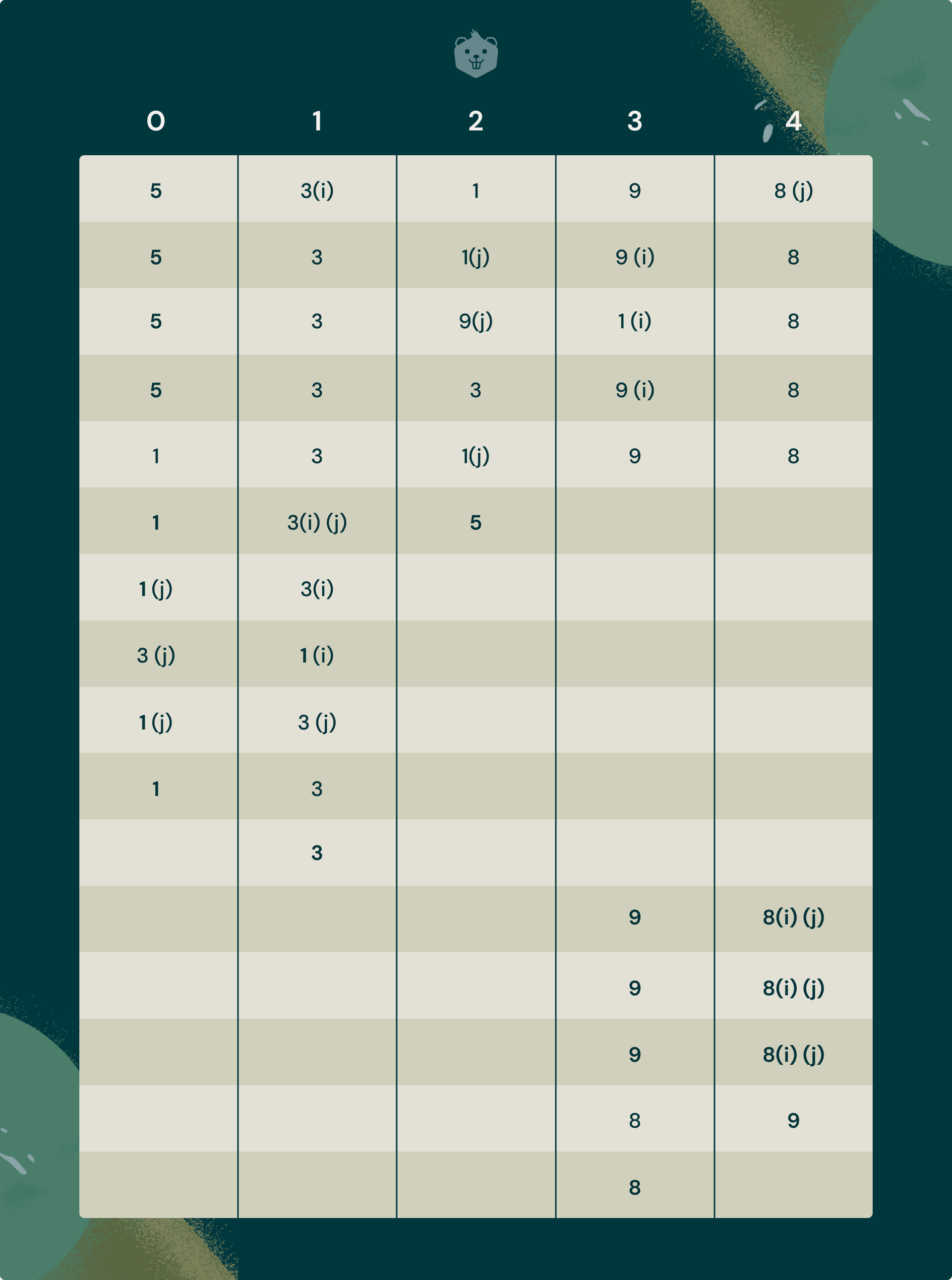
Using the algorithm you just learned for Partition, trace Partition for an array = [5, 3, 1, 9, 8]
Your trace of the array should look like the figure below. The highlighted elements are the pivots.
Here is a link to help you visualize Quick Sort


(select Quick Sort at the top)
Tree of recursive calls
Quick Sort will first recursively be called on the left half of the tree, then it will work on the right half.
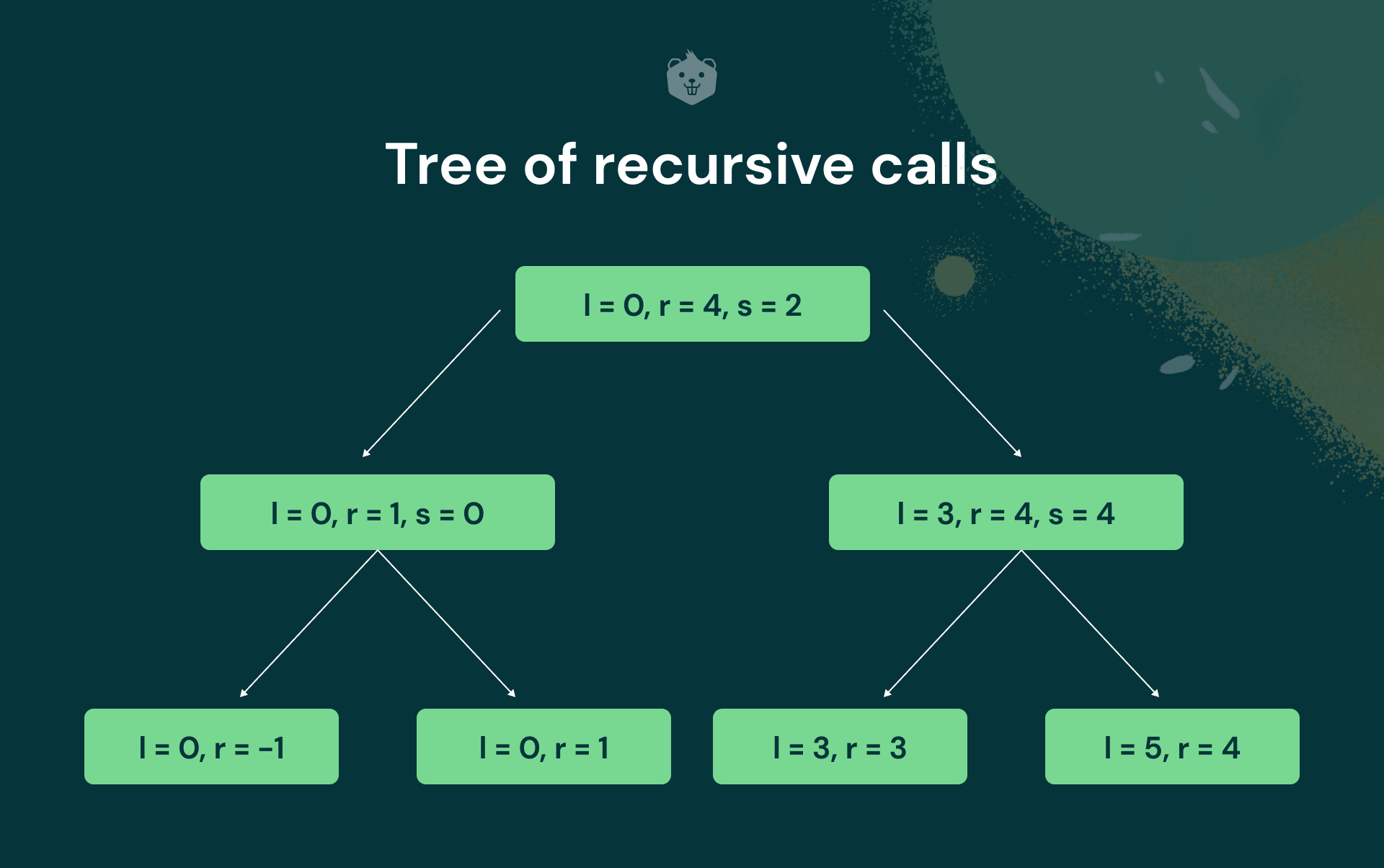
Here you can see that all the nodes in the last level do not satisfy the condition
l<r . So, no action is performed.
Implementation of Quick Sort in Python
# The main function that implements QuickSort
def quicksort(array, l, r):
if (l < r):
# s is partitioning index
#pivot will be placed in array[s]
s = partition(array,l , r)
# Sort elements before partition
# and after partition
quicksort(array,l, s - 1)
quicksort(array, s + 1, r)

#Partition function that sorts subarrays and returns partitioning index
def partition(array, l, r):
# Initializing pivot's index to start
i = l
pivot = array[l]
j = r+1
while(i=r or array[i]>=pivot):
break
while True:
j = j - 1
if(j<=l or array[j]<=pivot):
break
array[i], array[j] = array[j], array[i] #swap elements at i and j
array[i], array[j] = array[j], array[i] #undo last swap when i > j
array[l], array[j] = array[j], array[l]  #swap pivot and element at j

return j #return partition index

if __name__ == "__main__":
array = [9,8,7,6,5]
quicksort(array, 0, len(array) - 1)
print(f'Sorted array: {array}')
Output: Sorted array: [5, 6, 7, 8, 9]
Implementation of Quick Sort using random pivot
Randomized Quick Sort will make use of a random pivot that is selected randomly from the array, instead of choosing the first element as the pivot. This helps to avoid the worst case scenario of Quick Sort.
In this code, you will randomly select a pivot, and you will swap it with the first element.
import random
def randomized_partition(array, l, r):
i = l
pivot = random.randrange(l,r)
# Swap positions of randomly chosen pivot and the first element in the array
array[l], array[pivot] = array[pivot], array[l]

j = r+1
while(i=r or array[i]>=array[l]):
break

while True:
j = j - 1
if(j<=l or array[j]<=array[l]):
break
array[i], array[j] = array[j], array[i]
array[i], array[j] = array[j], array[i]
array[l], array[j] = array[j], array[l]

return j

def randomized_quicksort(array, l, r):
if (l < r):
s = randomized_partition(array,l , r)
randomized_quicksort(array,l, s - 1)
randomized_quicksort(array, s + 1, r)

if __name__ == "__main__":
array = [9,8,7,6,5]
randomized_quicksort(array, 0, len(array) - 1)
print(f'Sorted array: {array}')
Output:
Sorted array: [5,6,7,8,9]
Test your understanding
Q1. How does the array [5,2,4,9,1,9] look after the first partition?
Q2. Sorting in Quick Sort occurs within the same array
A.True
B. False
Q3. How do you make sure scan indices i and j don't go out of bound?
(Hint: Compare Quick Sort algorithm and Quick Sort Python code)
Q4. Why do we stop scanning when we find an element equal to the pivot?
Time Complexity Analysis

Best case
Quick Sort makes n + 1 key comparisons if scanning indices cross over. If not, then n comparisons are made. If all partitions occur at the middle of all subarrays, you have the best case scenario.
Cbest(n) = 2Cbest(n/2) + n for n > 1 , Cbest(1) = 0
C = number of comparisons made.
By applying masters theorem,
Cbest(n) = nlogn
Worst Case
The worst case scenario will occur when the array is already sorted. It could be sorted in increasing or decreasing order. All the splits, in this case, will occur at the extremes of the array, and at least one of the two subarrays will be empty.
It also occurs when all elements are the same.
Say you have an array that is sorted in increasing order as the input. The scan i will have to scan and compare elements with the pivot all the way till the end of the array.
First, it will make n + 1 comparisons. It will exchange the pivot element with itself. Now it will run the scan for A[1..n-1]. It will make n comparisons. Then it will scan for A[2..n-1]. It will make n - 1 comparisons, and so on.
Cworst(n) = (n+1) + n + …….. + 3 = (n+1)(n+2)/2
Which belongs to O(n2)
Time complexity comparison of Quick Sort and randomized Quick Sort
You just learned that the worst case time complexity of Quick Sort is O(n2). Randomized Quick Sort improves the performance.
The worst case time complexity is still O(n2), but the chances of it occurring are decreased.
Here you will pass a sorted array to functions quicksort, and randomized_quicksort, and see which one has a better running time.
import time
from random import randint
arr1 = [randint(0,1000) for i in range(1000)]
times=[]
times_worstcase = []
randomized_worstcase = []

for x in range(0,1000,10):
start_time = time.time()
arr2 = (arr1[:x])
quicksort(arr2,0, len(arr2)-1)
elapsed_time = time.time() - start_time
times.append(elapsed_time)
#store the sorted array in arr1, so that this imitates worst case scenario for Quick Sort
arr1 = arr2

for x in range(0,1000,10):
start_time = time.time()
arr2 = (arr1[:x])
quicksort(arr2,0, len(arr2)-1)
elapsed_time = time.time() - start_time
times_worstcase.append(elapsed_time)
arr1 = arr2
for x in range(0,1000,10):
arr2 = (arr1[:x])
start_time = time.time()
randomized_quicksort(arr2,0, len(arr2)-1)
elapsed_time = time.time() - start_time
randomized_worstcase.append(elapsed_time)
x=[i for i in range(0,1000,10)]

import matplotlib.pyplot as plt
%matplotlib inline
plt.xlabel("No. of elements")
plt.ylabel("Time required")
plt.plot(x,times_worstcase,'r')
plt.plot(x,randomized_worstcase,'b')
Output
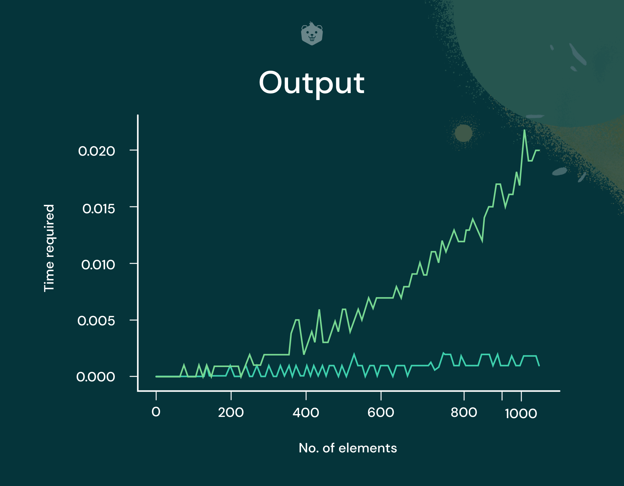
Observe that the running time plot for Quick Sort is leaning towards n2, while randomized_quicksort appears to have nlogn.
So even though a worst case input was passed to randomized_quicksort, it avoided the worst case by selecting a random pivot instead of the first element itself as the pivot.
Further Analysis of Quick Sort
The criteria for analyzing any sorting algorithm are the following:
Time complexity
The running time of Quick Sort heavily depends on the choice of the pivot element.
If worst case scenario does not occur in Quick Sort, its performance is comparable with merge sort. Quick Sort is one of the quickest sorting algorithms. Selection sort is the slowest.
Best case : O(nlogn)
Worst case: O(n2)
Average case: O(nlogn)
Space Complexity
Quick sort is an in-place sorting algorithm. It has a space complexity of O(1)
An in-place algorithm is a sorting algorithm in which the sorted items occupy the same storage as the original ones.
However, the worst case space complexity is O(logn).
Stability
Quick Sort is not a stable algorithm. An algorithm is said to be stable when it keeps elements with equal values in the same relative order in the output as they were originally, in the input.
Quick Sort works well on large data sets. Since it is in-place, it doesn't require additional memory.
Applications of Quick Sort
- Most commercial applications use Quick Sort to sort data. Data that is a mixture of different items can be assigned priorities and sorted. Miscellaneous data, such as student details, employee details, social media account profile sorting, sorting for e-commerce websites, etc.,
- Since Quick Sort works in-place, it is cache friendly
- It is used in Operations Research and Event Driven Simulation
- Amongst all the sorting algorithms which have an efficiency of nlogn, Quick Sort works best for sorting randomly ordered arrays.
- Java’s inbuilt Arrays.sort method uses dual pivot Quick Sort algorithm.
Test Your Understanding
Q4. Strictly decreasing arrays are
A. Worst-case input
B. Best-case input
C. Neither
Q5. Find out the worst case space complexity of Quick Sort. Why is this the case?
Q6. Which scenario is the best case for Quick Sort?
A.The elements are in ascending order
B.The pivot is the smallest element all of the time.
C.The elements are in random order
D.The elements are in alternating small/large order.
Q7. Quick Sort is the fastest sorting algorithm
A. True
B. False
Try it yourself
- Apply Quick Sort to sort the list L, E, A, R, N, B, Y, D, O, I, N, G in alphabetical order.
- Do a comparative study of Merge Sort and Quick Sort
- Write Quick Sort code with fewer swaps
Conclusion
Quick Sort is a heavily researched sorting algorithm as it can be improved in several ways based on how the pivot is chosen, and how the array is partitioned. It performs well on large data sets, and since it works in-place, it is sometimes a better alternative than merge sort. For a large data set of randomly organized numbers, Quick Sort does have a very low running time compared to other sorting algorithms like bubble sort and insertion sort. So yes! Quick Sort is pretty quick in sorting!
Further reading