Create a machine learning model using linear regression and Boston housing dataset while following the machine learning workflow.
Objective
Project Context
In machine learning we write computer programs which automatically improve with experience which are termed as machine learning models. It saves us from explicitly writing code for complex real world data.
In this project we are going to use supervised learning, which is a branch of machine learning where we teach our model by examples. Here we will first explore different attributes of Boston housing dataset then a part of dataset will be used to train the linear regression algorithm after that we will use the trained model to give predictions on remaining part of dataset.
Project Stages
The project consists of the following stages:
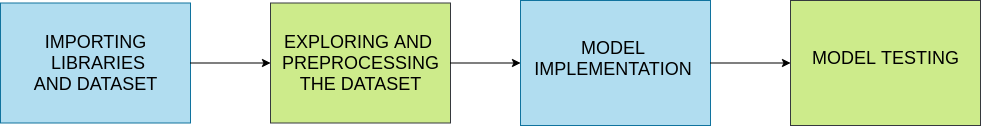
High-Level Approach
- Exploring and analyzing the data used for making prediction
- Creating a simple model using linear regression
- Using the model to carryout prediction and evaluating it's efficiency
Objective
Create a machine learning model using linear regression and Boston housing dataset while following the machine learning workflow.
Project Context
In machine learning we write computer programs which automatically improve with experience which are termed as machine learning models. It saves us from explicitly writing code for complex real world data.
In this project we are going to use supervised learning, which is a branch of machine learning where we teach our model by examples. Here we will first explore different attributes of Boston housing dataset then a part of dataset will be used to train the linear regression algorithm after that we will use the trained model to give predictions on remaining part of dataset.
Project Stages
The project consists of the following stages:
High-Level Approach
- Exploring and analyzing the data used for making prediction
- Creating a simple model using linear regression
- Using the model to carryout prediction and evaluating it's efficiency
Importing libraries and dataset
In this section we will load a few libraries which we will need to develop, visualize and test our model. We will also be loading our dataset for one of the imported libraries named Sklearn.
Requirements
-
To start right away search on Google for "Google colab", click on the first link and then click on new notebook. [Colab is a cloud based environment which provides all the resources required for model development.]
-
Import the stated libraries:
-
Numpy
-
Pandas
-
Sklearn
-
matplotlib.plt
-
Seaborn
-
-
Import Boston housing dataset from Sklearn using the following command.
from sklearn.datasets import load_boston
var = load_boston()
A bunch object is returned by load_boston() on which we will do our further work.
References
Tip
Run the command %matplotlib inline to get the view of plots in notebook itself.
Bring it On!
- Instead of load_boston() method try to load the dataset in colab notebook as a CSV file after downloading it from it's source mentioned above.
- Try to load from local disk as well as from a URL.
Expected Outcome
- Required libraries should be imported as well as the dataset from Sklearn
print(var.keys())should return a dictionary
Data exploration and preprocessing
In this section we will analyse our dataset using different methods and then we'll create a dataframe using the same. We will also carry out preprocessing on the dataframe for using the linear regression model.
Requirements
-
Use print statement on each element of dictionary returned by the above statement and read the results Ex:
print(var.DESCR)to understand the dataset. -
Create a pandas dataframe for creating a copy of the dataset on which we will carry out further preprocessing. Use the following command:
df = pd.DataFrame(var.data, columns=var.feature_names) -
Checkout references available below to know more about other arguments which can be used in
DataFrame()function. -
Use functions
head()andtail()to see first and last five rows of the created dataframe. -
Use
describe()to get even further insights on the created data frame. -
Add another column to the dataframe and store the value of target attribute in it
df['MEDV'] = var.targetConfirm the addition of column usinghead(). -
Use
df.dtypeordf.infoto know data type various features present in the dataset. If we find categorical data, then we'll require to use different encoding methods. -
Use
df.isnull().sum()to check for missing values in each column. If we find missing values, then either we will place values there or we can drop the row or column. -
Create a box plot using
seabornto see the outliers in the dataset. Generally we remove the rows having outliers from our data but for small dataset like Boston housing it can lead to a loss of a significant percentage of data.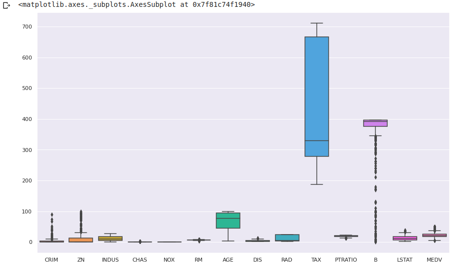
-
Create a heatmap using
seabornto find corelation between different features and labels. In model creation we will be using features having a high corelation with our target label.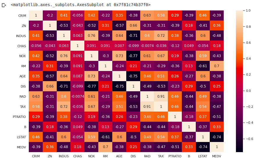
-
Create
KDEplot of different variables usingseabornlibrary.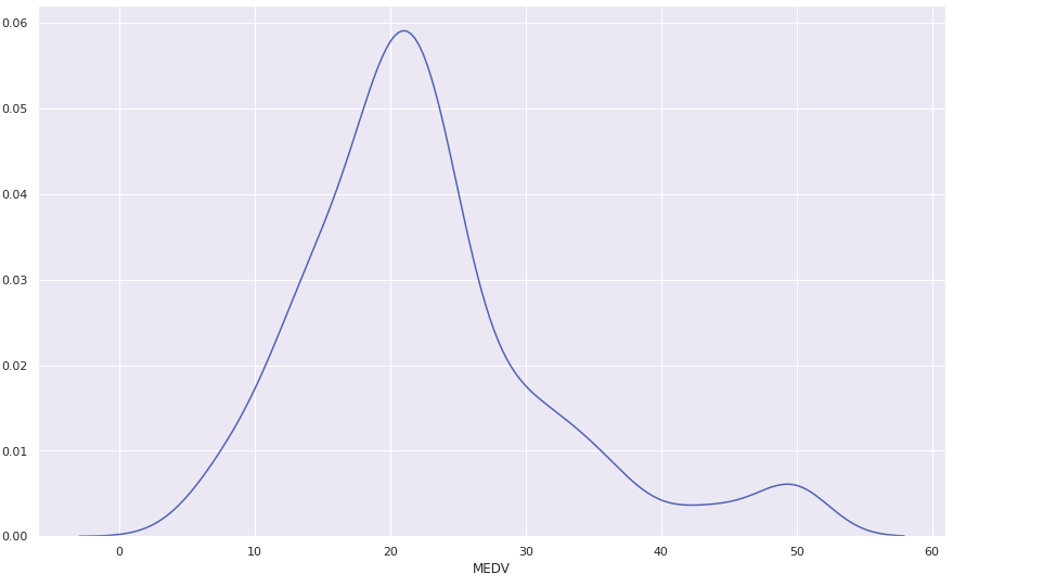
Bring it On!
- In normalization we rescale numeric values of attributes to the range [1,0]. Create another dataframe and perform all the above steps followed by normalization of data.
- After model implementation check the effect of normalization on the accuracy of the model
- Instead of heatmap try to create a bar graph to identify collinearity.
Expected Outcome
- On completion of this milestone, you should be able to achieve the following:
- A dataframe being created and a new column having value of target being added to it .
- Data being observed and understood using different methods
- Different aspects of data being visualized for a better understanding.
- Using heatmap features having high corelation with the target label had been identified.
Model Implementation
In this section we will import linear regression model from Sklearn. Use features identified from heatmap and label to create training and testing set. Finally we will train our model using training set.
Requirements
-
Select features for creating training and test set. In place of variable x put your features (for example, NOX which stands for Nitric Oxide content) and MEDV (Median value) as a label in y
x1 = bdf[['NOX','RM','DIS','PTRATIO','LSTAT' ]] y1 = bdf['MEDV'] -
Use train_test split() from Sklearn to create train and test sets
x_train, x_test, y_train, y_test = train_test_split(X1, Y1, test_size =0.33,random_state = 5 ) -
Use regression on training data
regressor = LinearRegression()
regressor.fit(x_train, y_train)
y_pred = regressor.predict(x_test)
df = pd.DataFrame({'Actual': y_test, 'Predicted': y_pred})
df
References
Tip
- In case of error in using the functions we can directly import the required functions.
from sklearn.model_selection import train_test_split
from sklearn.linear_model import LinearRegression
from sklearn import metrics
Bring it On!
- Try to use SVM Regressor and Random Forest Regressor for model creation on normalized dataframe, and compare the respective R2 scores.
Expected Outcome
- You should be able to achieve the following:
- Create training and test set from the dataframe.
- Train the model using the training set and display the predicted and actual values.
Model Testing
In this section we will test our prediction with testing data and calculate R2 score to measure model accuracy. We will also plot the results of the linear regression model.
Requirements
- Display the following: Mean Absolute Error, Mean Squared Error, Root Mean Squared Error, R2 Score.
metrics.mean_absolute_error()
metrics.mean_squared_error()
np.sqrt(metrics.mean_squared_error())
metrics.r2_score()
The above code block is missing some arguments. Checkout the references to get a clear idea on what it's missing.
-
Use array function in
numpyto crate an array of target label and any one of the features. Pass this throughpolyfit()function.polyfit()will return the slope and intercept of regression line. Store the returned values.x1 = numpy.array(x_test['NOX']) y1 = numpy.array(y_pred) m,b=numpy.polyfit()The above code snippet is missing arguments for
polyfit(). Checkout the references for a solution. -
Use the
plot()function to plot the regression line corresponding to the chosen feature.plt.plot(x_test['NOX'], m*x_test['NOX'] + b) plt.plot(x_test['NOX'],y_pred,'o') plt.xlabel("Nitric Oxide Content") plt.ylabel("Median Value")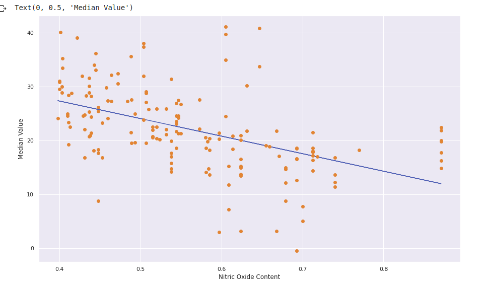 Read about the functions and it's argument in the references section.
 -
Use
seabornlibrary to create apairplotsns.pairplot(bdf, x_vars=['NOX','RM','DIS','PTRATIO','LSTAT'], y_vars='MEDV', height=9, aspect=0.6, kind='reg')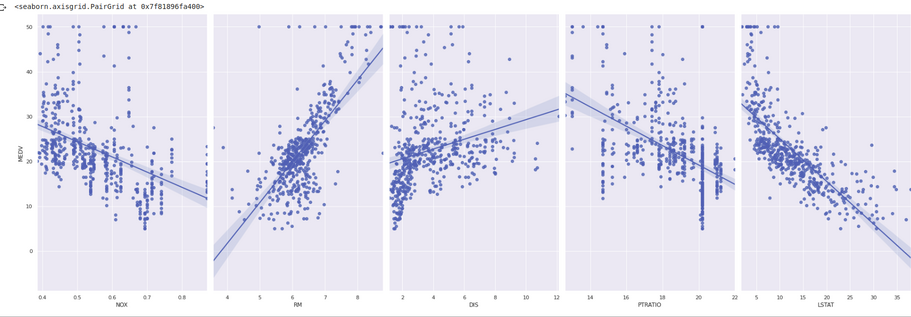
Read about the function and its arguments from references to know more about
pairplotand try to play around with various argument values.
Bring it On!
- Use other features to create their plots with predicted values.
Expected Outcome
- You should be able to achieve the following:
- Display and interpret the R2 score and results of error functions
- Create and display a plot using negative slope and positive y intercept obtained from
polyfit()function for Median value label and Nitric oxide content attribute. - Create and display a
pairplotof the attributes against the label where attributes with positive corelation with the label will have plots with positive slope and attributes having negative corelation will have negative slope.