What is time complexity?
Time complexity is a programming term that quantifies the amount of time it takes a sequence of code or an algorithm to process or execute in proportion to the size and cost of input.
It will not look at an algorithm's overall execution time. Rather, it will provide data on the variation (increase or reduction) in execution time when the number of operations in an algorithm increases or decreases.
Yes, as the definition suggests, the amount of time it takes is solely determined by the number of iterations of one-line statements inside the code.
Take a look at this piece of code:
Although there are three separate statements inside the main() function, the overall time complexity is still O(1) because each statement only takes unit time to complete execution.
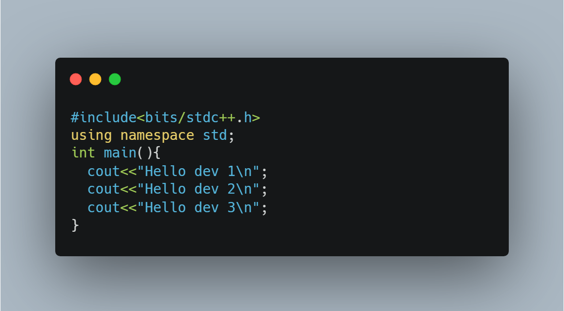
Whereas, observe this example:
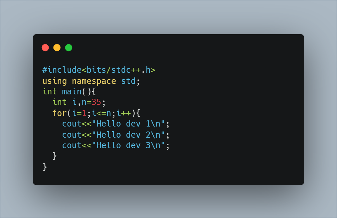
Here, the O(1) chunk of code (the 3 cout statements) is enclosed inside a looping statement which repeats iteration for 'n' number of times. Thus our overall time complexity becomes n*O(1), i.e., O(n).
You could say that when an algorithm employs statements that are only executed once, the time required is constant. However, when the statement is in loop condition, the time required grows as the number of times the loop is set to run grows.
When an algorithm has a mix of single-executed statements and LOOP statements, or nested LOOP statements, the time required increases according to the number of times each statement is run.
For example, if a recursive function is called multiple times, identifying and recognizing the source of its time complexity may help reduce the overall processing time from 600 ms to 100 ms, for instance. That's what time complexity analysis aims to achieve.
Understanding various Time Complexity notations
The following are some of the most common asymptotic notations for calculating an algorithm's running time complexity;
- Ο Notation
- Ω Notation
- θ Notation
Before you dig in, don't miss to check out the top 10 sorting algorithms used
Big Oh Notation, Ο
The systematic way to express the upper limit of an algorithm's running time is to use the Big-O notation O(n). It calculates the worst-case time complexity, or the maximum time an algorithm will take to complete execution.
Also, do remember that this is the most commonly used notation for expressing the time complexity of different algorithms unless specified otherwise.
Definition:
Let g and f be functions that belong to the set of natural numbers (N). The function f is said to be O(g), if there is a constant c > 0 and a natural number n0 such that:
f (n) ≤ cg(n) for all n >= n0Omega Notation, Ω
The systematic way to express the lower bound of an algorithm's running time is to use the notation Ω(n). It calculates the best-case time complexity, or the shortest time an algorithm will take to complete.
Definition:
Ω(g(n)) ={ f(n): there exist positive constants c and n0 such that 0 ≤ cg(n) ≤ f(n) for all n ≥ n0 }The above expression can be defined as a function f(n) which belongs to the set Ω(g(n)) if and only if there exists a positive constant c (c > 0) such that it is greater than c*g(n) for a sufficiently large value of n.
The minimum time required by an algorithm to complete its execution is given by Ω(g(n)).
Theta Notation, Θ
The systematic way to express both the lower limit and upper bound of an algorithm's running time is to use the notation (n).
Definition:
Θ(g(n)) = {f(n): there exist certain positive constants x1, x2 and n0 such that 0 ≤ x1g(n) ≤ f(n) ≤ x2g(n) for all n ≥ n0}Why should you learn about the time complexity of algorithms?
In computer programming, an algorithm is a finite set of well-defined instructions that are usually performed in a computer to solve a class of problems or perform a common operation.
According to the description, a sequence of specified instructions must be provided to the machine for it to execute an algorithm or perform a specific task. A particular series of instructions may be interpreted in any number of ways to perform the same purpose.
We have mentioned that the algorithm is to be run on a computer, which leads to the next step of varying the operating system, processor, hardware, and other factors that can affect how an algorithm is run.
Now that you know that a variety of variables will affect the outcome of an algorithm, it's important to know how effective those algorithms are at completing tasks. To determine this, you must assess an algorithm's Space and Time complexity.
An algorithm's space complexity quantifies how much space or memory it takes to run as a function of the length of the input while an algorithm's time complexity measures how long it takes an algorithm to run as a function of the length of the input.
That's why it's so important to learn about the time and space complexity analysis of various algorithms.
Let's explore each time complexity type with an example.
1. O(1)
Where an algorithm's execution time is not based on the input size n, it is said to have constant time complexity with order O (1).
Whatever be the input size n, the runtime doesn’t change. Here's an example:
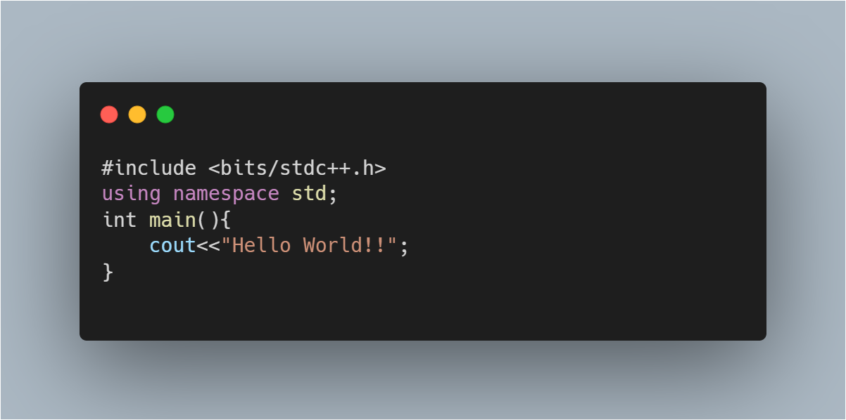
As you can see, the message "Hello World!!" is printed only once. So, regardless of the operating system or computer configuration you are using, the time complexity is constant: O(1), i.e. any time a constant amount of time is required to execute code.
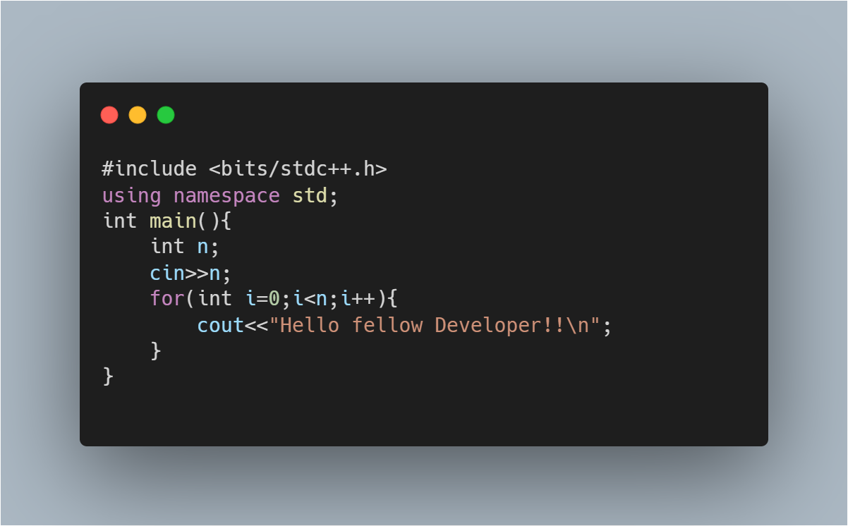
2. O(n)
When the running time of an algorithm increases linearly with the length of the input, it is assumed to have linear time complexity, i.e. when a function checks all of the values in an input data set (or needs to iterate once through every value in the input), it is said to have a Time complexity of order O (n). Consider the following scenario:
Output:
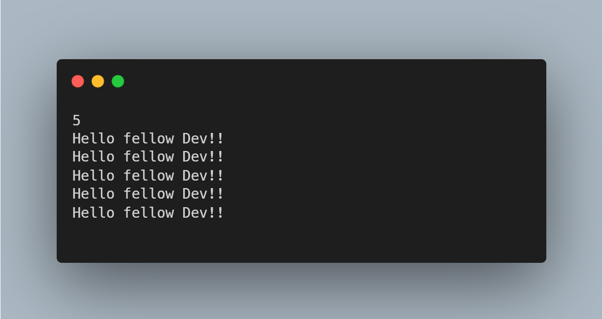
Based on the above code, you can see that the number of times the statement "Hello fellow Developer!!" is displayed on the console is directly dependent on the size of the input variable 'n'.
If one unit of time is used to represent run time, the above program can be run in n times the amount of time. As a result, the program scales linearly with the size of the input, and it has an order of O(n).
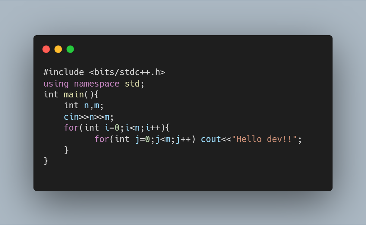
3. O(n^2)
When the running time of an algorithm increases non-linearly O(n^2) with the length of the input, it is said to have a non-linear time complexity.
In general, nested loops fall into the O(n)*O(n) = O(n^2) time complexity order, where one loop takes O(n) and if the function includes loops inside loops, it takes O(n)*O(n) = O(n^2).
Similarly, if the function has ‘m' loops inside the O(n) loop, the order is given by O (n*m), which is referred to as polynomial time complexity function.
Consider the following program:
Output:
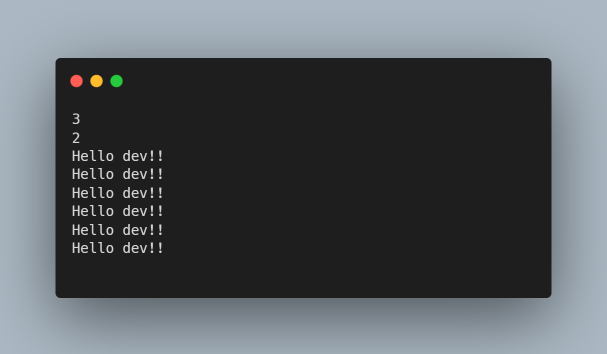
As you can see, there are two nested for loops such that the inner loop's complete iteration repeats based on the value of the outer loop. This is the primary reason why you see "Hello dev!!" printed 6 times (3*2).
This amounts to the cumulative time complexity of O(m*n) or O(n^2) if you assume that the value of m is equal to the value of n.
4. O(log2 n)
When an algorithm decreases the magnitude of the input data in each step, it is said to have a logarithmic time complexity. This means that the number of operations is not proportionate to the size of the input.
O (log2 n) basically implies that time increases linearly while the value of 'n' increases exponentially. So, if computing 10 elements take 1 second, computing 100 elements takes 2 seconds, 1000 elements take 3 seconds, and so on.
When using divide and conquer algorithms, such as binary search, the time complexity is O(log n).
Another example is quicksort, in which we partition the array into two sections and find a pivot element in O(n) time each time. As a result, it is O(log2 n)
Binary trees and binary search functions are examples of algorithms having logarithmic time complexity. Here, the search for a particular value in an array is done by separating the array into two parts and starting the search in one of them. This guarantees that the action isn't performed on every data element.
Consider the following code snippet:
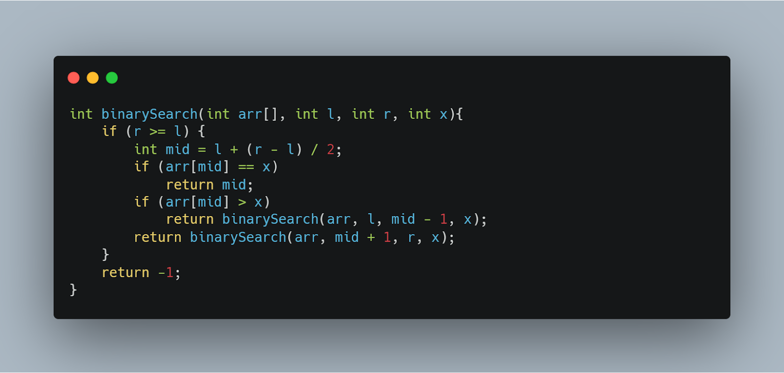
The above program is a demonstration of the binary search technique, a famous divide-and-conquer approach to searching in logarithmic time complexity.
Time Complexity Analysis
Let us assume that we have an array of length 32. We'll be applying Binary Search to search for a random element in it. At each iteration, the array is halved.
- Iteration 0:
- Length of array = 32
- Iteration 1:
- Length of array = 32/2 = 16
- Iteration 2:
- Length of array = 32/2^2 = 8
- Iteration 3:
- Length of array = 32/2^3 = 4
- Iteration 4:
- Length of array = 32/2^4 = 2
- Iteration 5:
- Length of array = 32/2^5 = 1
Another example would be that for an array of size 1024, only 10 iterations are needed to approach unity. For an array size of 32768, we'll need only 15 iterations. Thus we can see that the number of operations grows at a very small rate compared to the size of the input array while complexity is logarithmic.
To generalize, after k iterations, our array size approaches 1.
Hence, n/2^k = 1 => n = 2^k
Applying logarithmic function on both sides, we get
=> log2 (n) = log2 (2^k) => log2 (n) = k log2 (2)
or, => k = log2 (n)
Hence, the time complexity of Binary Search becomes log2(n), or O(log n)
5. O (n log n)
This time complexity is popularly known as linearithmic time complexity. It performs slightly slower as compared to linear time complexity but is still significantly better than the quadratic algorithm.
Consider the program snippet given below:
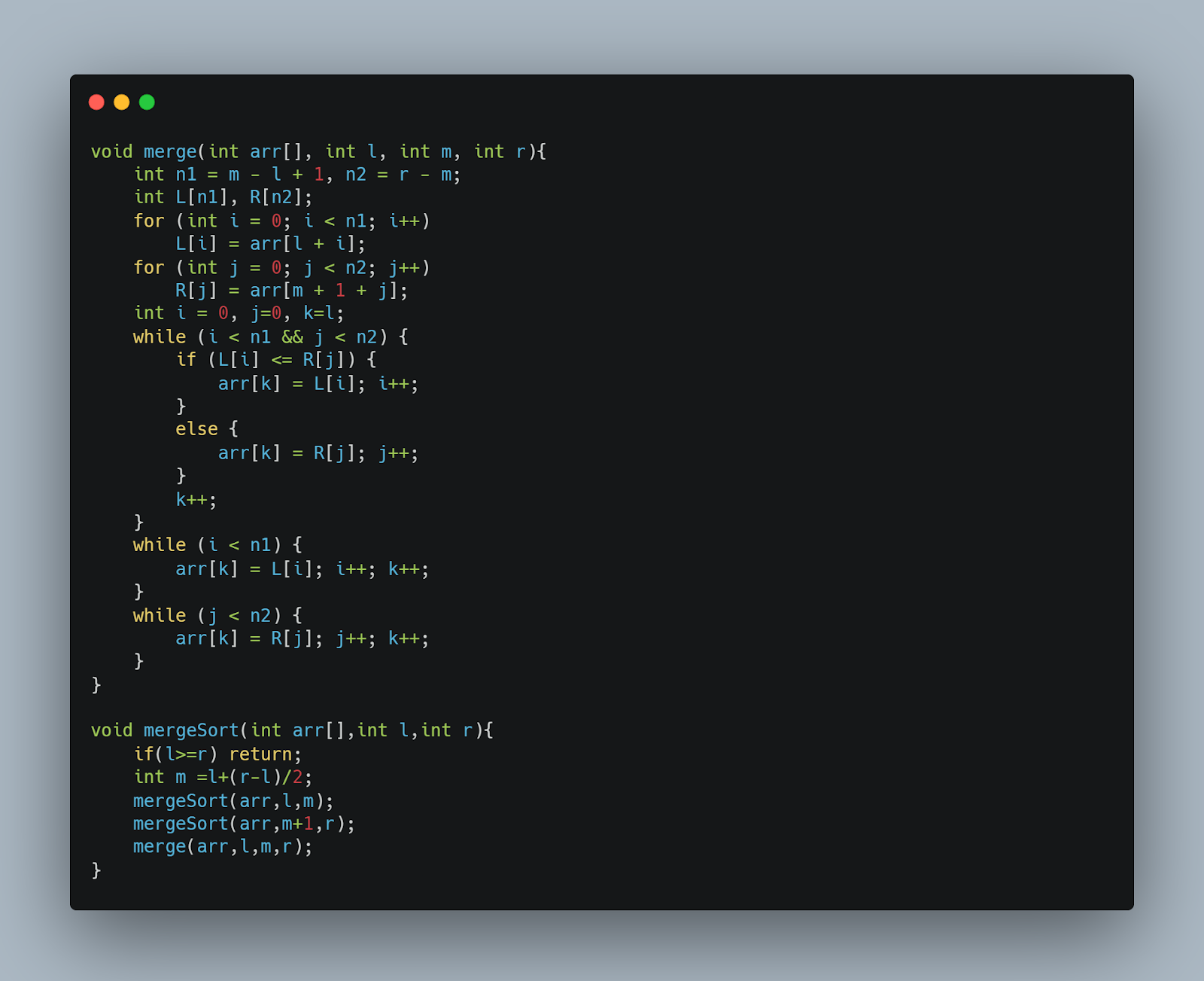
The program above represents the merge sort algorithm.
Sorting arrays on separate computers take a significant time. Merge Sort algorithm is recursive and has a recurrence relation for time complexity as follows:
T(n) = 2T(n/2) + θ(n)The Recurrence Tree approach or the Master approach can be used to solve the aforementioned recurrence relation.
It belongs to Master Method Case II, and the recurrence answer is O(n*logn). Since Merge Sort always partitions the array into two halves and merges the two halves in linear time, it has a time complexity of (n*logn) in all three circumstances (worst, average, and best).
Also, remember this, when it comes to sorting algorithms, O(n*logn) is probably the best time complexity we can achieve.
6. O(2^N)
An algorithm with exponential time complexity doubles in magnitude with each increment to the input data set. If you're familiar with other exponential growth patterns, this one works similarly. The time complexity begins with a modest level of difficulty and gradually increases till the end.
The Fibonacci series is a great way to demonstrate exponential time complexity. Given below is a code snippet that calculates and returns the nth Fibonacci number:

Time Complexity Analysis:
The recurrence relation for the above code snippet is:
T(n) = T(n-1) + T(n-2)Using the recurrence tree method, you can easily deduce that this code does a lot of redundant calculations as shown below.
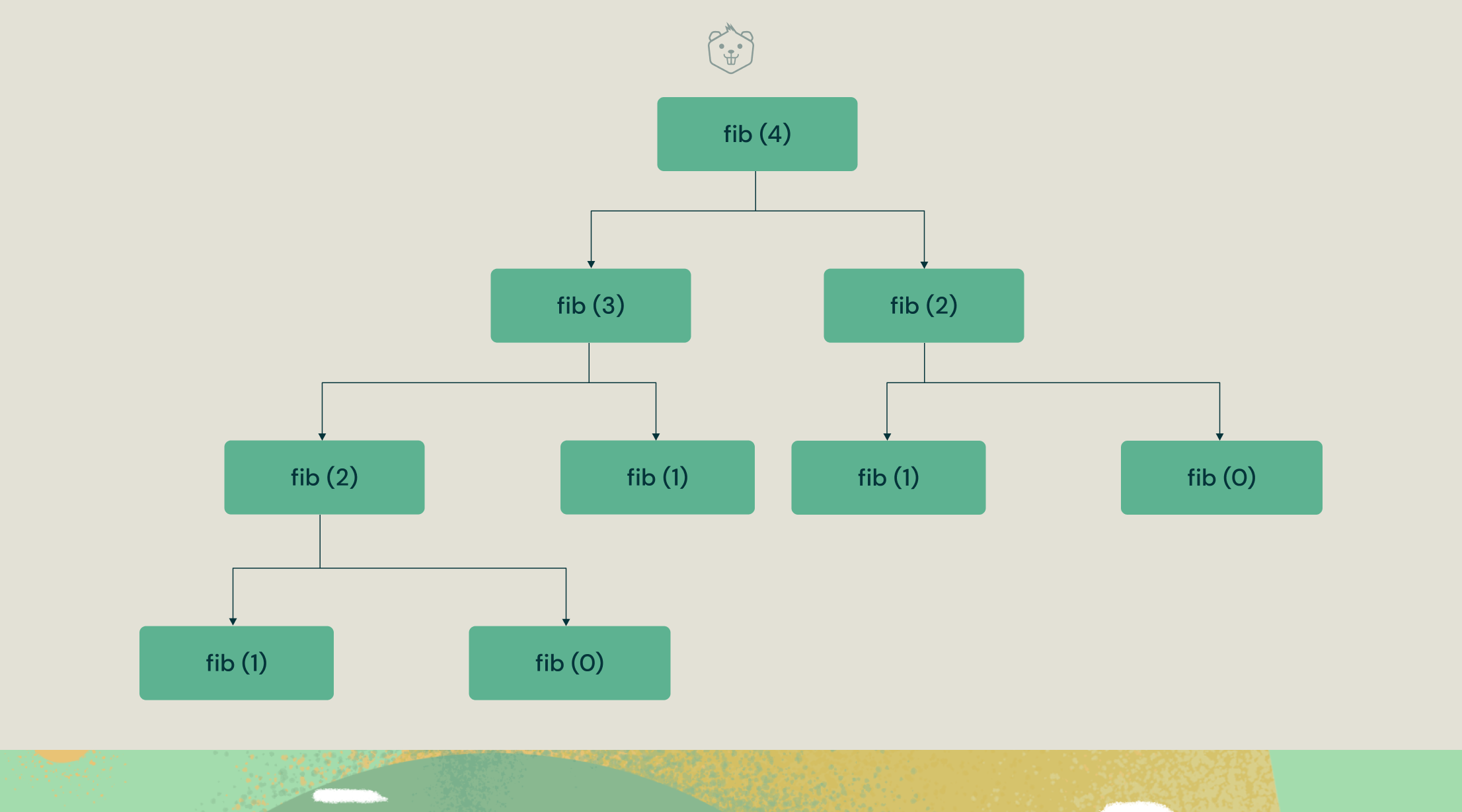
Thus the time complexity of the Fibonacci series becomes exponential owing to these repetitive calculations.
Let's take an example here to drive home the magnitude of this time complexity.
For n=3, it takes 8 operations to calculate the 8th Fibonacci number.
For n=4, it takes 16 operations
.
.
For n=10, it takes 1024 operations to reach the 10th Fibonacci number.
.
.
Now if we bump it up to 100 (n=100), we literally exceed billions and billions of calculations just to reach the 100th Fibonacci number.
That's scary right. That's why exponential time complexity is one of the worst time complexities out there.
Now that you've explored the major time complexities in algorithms and data structures, take a look at their graphical representation below: (Time vs Input Size)
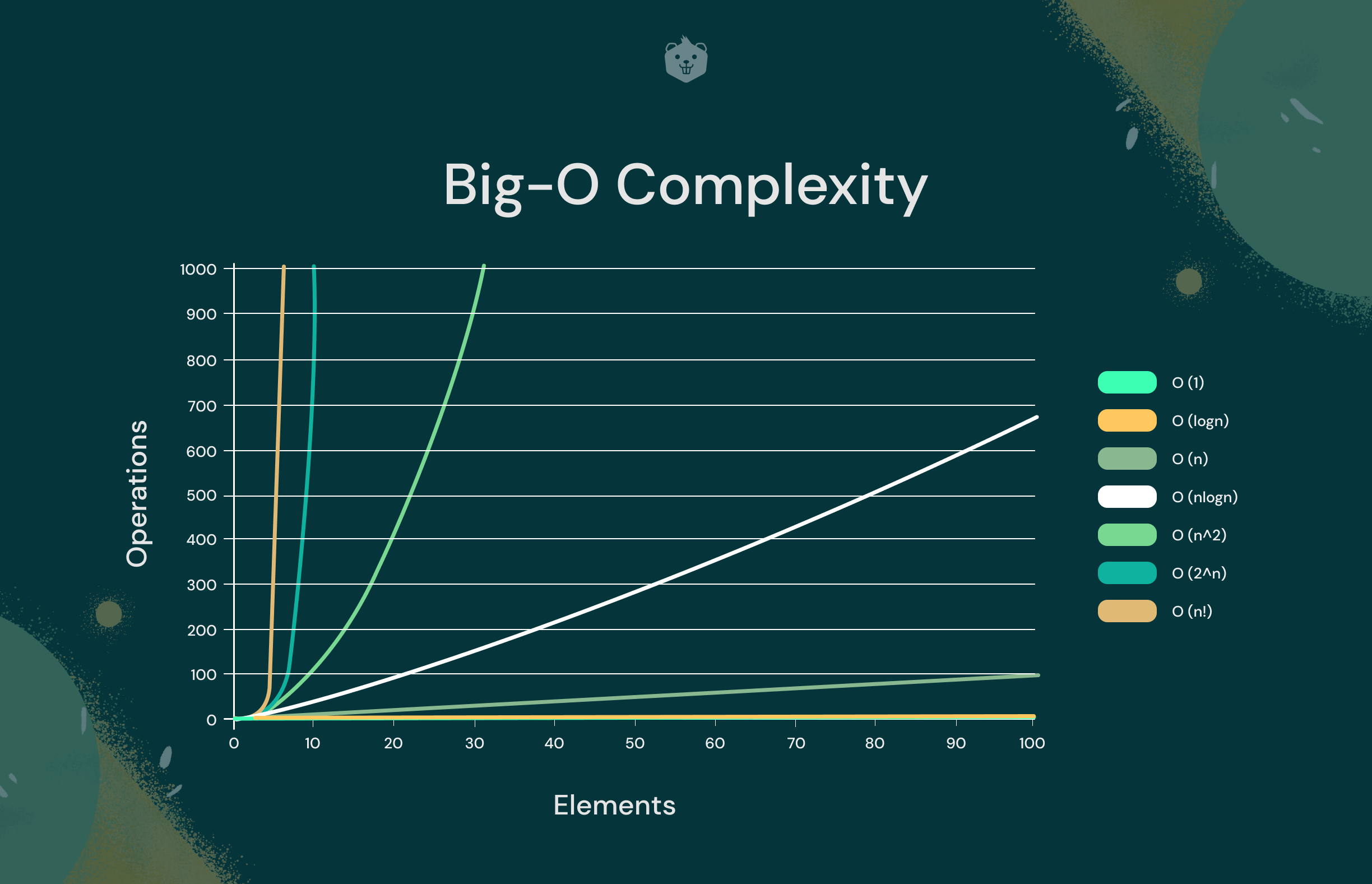
Here's a simple comparison between different time complexities to help you understand the graph better:
O(1) < O(log2n) < O(n1/2) < O(n) < O(n logn) < O(n^2) < O(n^3) < . . . . < O(2^n) < O(3^n) < . . . . < O(n^n)Of course, a visual representation clarifies a lot of concepts particularly related to the efficiency of different time complexities.
The noticeable thing to observe is how inefficient exponential and quadratic time complexities are with increasing input data size.
On the other hand, linearithmic and linear time complexities perform almost in a similar fashion with increasing input size.
The astounding part is the performance of logarithmic time complexity which clearly supersedes most algorithmic time complexities (except O(1)) in terms of execution time and efficiency.
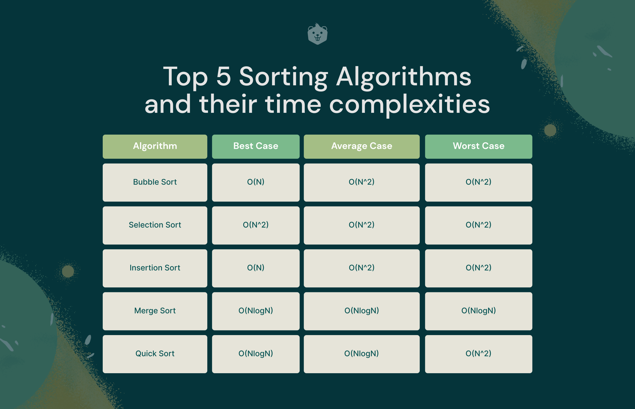
Top 5 Sorting Algorithms and their time complexities
HEY, seems like you just completed learning about one of the most important concepts in Data Structures and Algorithms, i.e, time complexity analysis. Hope you enjoyed this code-based approach to such an interesting topic.
With DSA it becomes important to identify the Time Complexity of a given piece of code in the long run.
You can always jumpstart with the knowledge here and put it into practice analyzing various code snippets to up your Time Complexity game.
Of course, it will take time, but the experience you'll gain out of that will be more potent than just skimming through this article. So, what are you waiting for? Go ahead and crunch out some awesome problems for yourself.
Any particular time complexity that we missed out on? Let us know in the comments below.
Also, if you learned something new at any point in this article, please spread the knowledge by sharing it with your friends or with someone who might need it.
HAPPY CODING!!