Before you begin..
Try giving a shot at common MAANG Sorting Algorithms Interview Questions before reading the blog.
Answer MAANG Interview QuestionsAfter you read the blog..
Answer more advanced questions to be absolutely interview-ready. Check out the quiz at the end. Read this blog to get a perfect score in that quiz :)
The arrangement of data in a specific order (ascending or descending) is termed sorting in data structures. Sorting data makes it easier to search through a given data sample, efficiently and quickly.
Why are Sorting Algorithms Important?
Since sorting can often help reduce the algorithmic complexity of a problem, it finds significant uses in computer science.
A quick Google search reveals that there are over 40 different sorting algorithms used in the computing world today. Crazy right?
Well, you will be flabbergasted when you realize just how useful sorting algorithms are in real life. Some of the best examples of real-world implementation of the same are:
- Bubble sorting is used in programming TV to sort channels based on audience viewing time!
- Databases use external merge sort to sort sets of data that are too large to be loaded entirely into memory!
- Sports scores are quickly organized by quick sort algorithm in real-time!!
How well do you know your sorting algorithms? Take this quiz to find out >>
Types of Sorting in Data Structures
Want to brush up your sorting algorithms before an interview? Answer these questions before you go >>
- Comparison-based sorting: In comparison-based sorting techniques, a comparator is defined to compare elements or items of a data sample. This comparator defines the ordering of elements. Examples are: Bubble Sort, Merge Sort.
- Counting-based sorting: There's no comparison involved between elements in these types of sorting algorithms but rather work on calculated assumptions during execution. Examples are : Counting Sort, Radix Sort.
- In-Place vs Not-in-Place Sorting: In-place sorting techniques in data structures modify the ordering of array elements within the original array. On the other hand, Not-in-Place sorting techniques use an auxiliary data structure to sort the original array. Examples of In place sorting techniques are: Bubble Sort, Selection Sort. Some examples of Not in Place sorting algorithms are: Merge Sort, Quick Sort.


This article will enable your problem solving skills with the Top 10 Sorting Algorithms used in the computing world today including bubble sort and merge sort algorithms.
You will also be diving deep into the working of various sorting techniques with intuitive examples covering time and space complexities in best and worst-case scenarios.

Finally, we'll wrap up with a broad-spectrum analysis as to which algorithm stands out in terms of time and space complexities.
Sorting Algorithms in Java vs C++
Java is the most popular language of choice when it comes to implementing algorithms and working with data structures in the software industry.
Level up your foundational programming skills in Java and practice the most relevant Data Structure questions in Crio's Backend Developer Program. Check out the full syllabus here >>
Although this blog focuses heavily on C++ based implementations, don't fret because as long as your logical understanding of these algorithms is strong, the only thing holding you back is basic syntactic differences between Java and C++.
Want to build your foundations of Java concepts? Check out these free immersive activities on Crio's learning platform >>
So without further ado, let's dive right in.
Need guidance with problem-solving and data structures? Go through Crio's Data Structures Track and unlock what it takes to tackle unseen problems with ease.
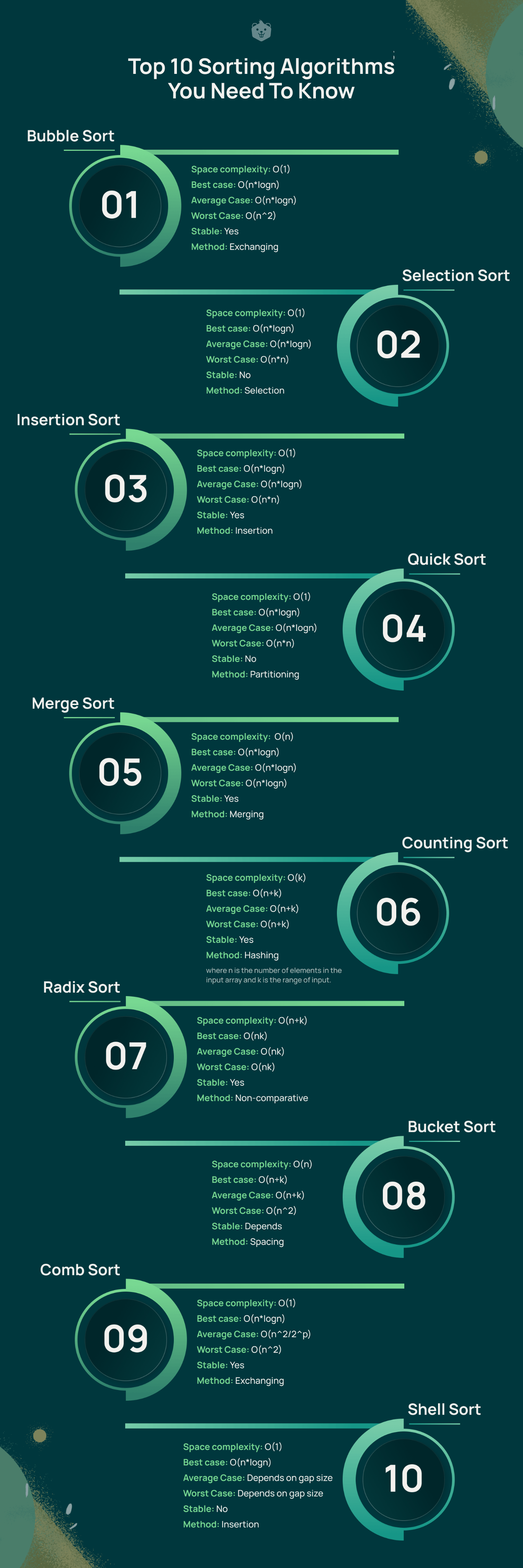
Top 10 Sorting Algorithms You Need To Know
1. Bubble Sort
The basic idea of bubble sorting is that it repeatedly swaps adjacent elements if they are not in the desired order. YES, it is as simple as that.
If a given array of elements has to be sorted in ascending order, bubble sorting will start by comparing the first element of the array with the second element and immediately swap them if it turns out to be greater than the second element, and then move on to compare the second and third element, and so on.
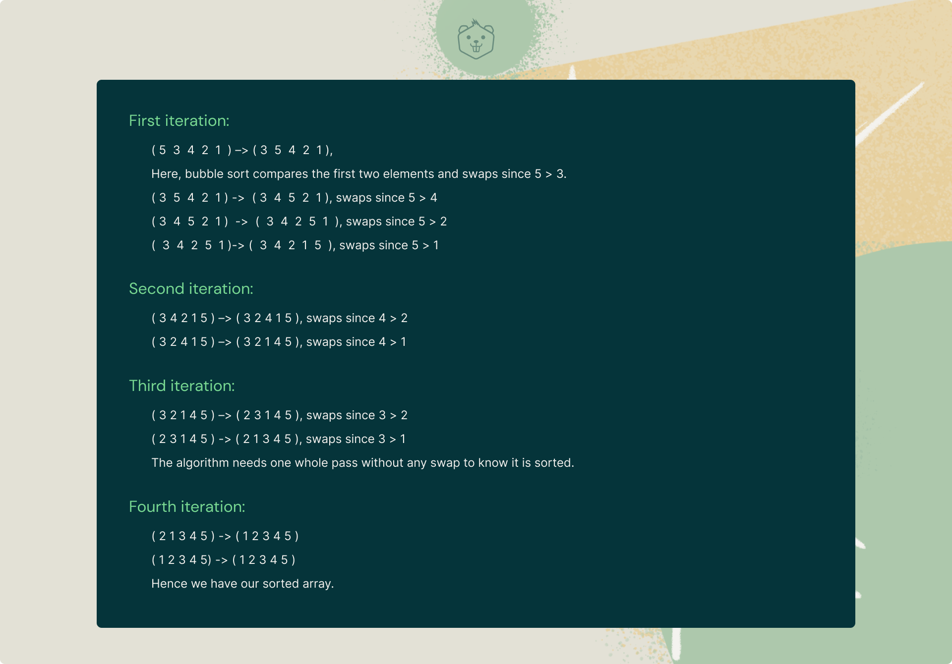
Understanding Bubble Sort algorithm with a simple example
Let's try to understand the intuitive approach behind bubble sort with an example:
Now that you've understood the intuitive idea behind bubble sort, it's time to take a look at its standard C++ implementation.
Implementation in C++
#include <bits/stdc++.h>
using namespace std;

void Bubble_Sort(int vec[], int n){
	int i, j;
	for (i = 0; i < n-1; i++)
	for (j = 0; j < n-i-1; j++)
		if (vec[j] > vec[j+1])
			swap(vec[j], vec[j+1]);
}
int main(){
	int vec[] = {5, 3, 4, 2, 1};
	int n = sizeof(vec)/sizeof(vec[0]);
	Bubble_Sort(vec, n);
	cout<<"Sorted array: \n";
	for (int i = 0; i < n; i++)
		cout << vec[i] << " ";
	cout << endl;
}Time Complexity:
- Worst Case: O(n^2)
- Average Case: O(n*logn)
- Best case: O(n*logn)
Auxiliary Space Complexity: O(1)
Also read: Time Complexity Simplified with Easy Examples
Use Cases
- It is used to introduce the concept of a sorting algorithm to Computer Science students.
- In computer graphics, bubble sorting is quite popular when it comes to detecting a very small error (like swap of just two elements) in almost-sorted arrays.
Try it yourself
Q. Given an array of n input integers, return the sum of maximum and minimum elements of the array. [Constraint: Use Bubble Sorting]
Input:
- n -> Size of array (n>1)
- 'n' array elements below
Output: A single line representing the required sum
P.S: Don't forget to drop a comment below if you face issues with this problem.
2. Selection Sort
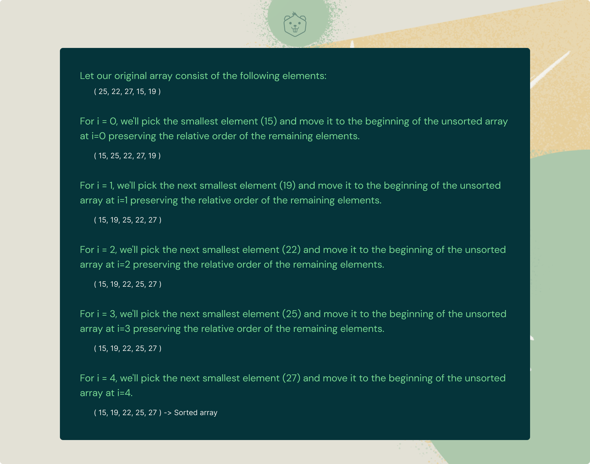
Selection sort is a sorting algorithm in which the given array is divided into two subarrays, the sorted left section, and the unsorted right section.
Initially, the sorted portion is empty and the unsorted part is the entire list. In each iteration, we fetch the minimum element from the unsorted list and push it to the end of the sorted list thus building our sorted array.
Still a bit fuzzy? Take a look at this awesome example below.
Understanding Selection Sort algorithm with an example
Let's try to understand the intuitive idea behind selection sort with a simple example:
Seems easy right? Because it is.
Now go ahead and take a look at its basic C++-based implementation.
#include <bits/stdc++.h>
using namespace std;

void Selection_Sort(int vec[], int n){
	int i, j, pos;
	for (i = 0; i < n-1; i++){
		pos = i;
		for (j = i+1; j < n; j++)
		if (vec[j] < vec[pos])
			pos = j;
		swap(vec[pos], vec[i]);
	}
}

int main(){
	int vec[] = {25, 22, 27, 15, 19};
	int n = sizeof(vec)/sizeof(vec[0]);
	Selection_Sort(vec, n);
	cout << "Sorted array: \n";
	for (int i=0; i < n; i++)
		cout << vec[i] << " ";
	cout << endl;
	return 0;
}Time Complexity:
- Worst Case: O(n*n)
- Average Case: O(n*logn)
- Best case: O(n*logn)
Auxiliary Space Complexity: O(1)
Also read: Time Complexity Simplified with Easy Examples
Use Cases
- It is used when the size of a list is small. (Time complexity of selection sort is O(N^2) which makes it inefficient for a large list.)
- It is also used when memory space is limited because it makes the minimum possible number of swaps during sorting.
Try it yourself
Q. Given an array of n input integers, return the absolute difference between the maximum and minimum elements of the array. [Constraint: Use Selection Sorting]
Input:
- n -> Size of array (n>1)
- 'n' array elements below
Output: A single line representing the required difference
Build 5 mini-projects and master essential data structures and algorithms you need to crack your next big tech interview.
3. Insertion Sort
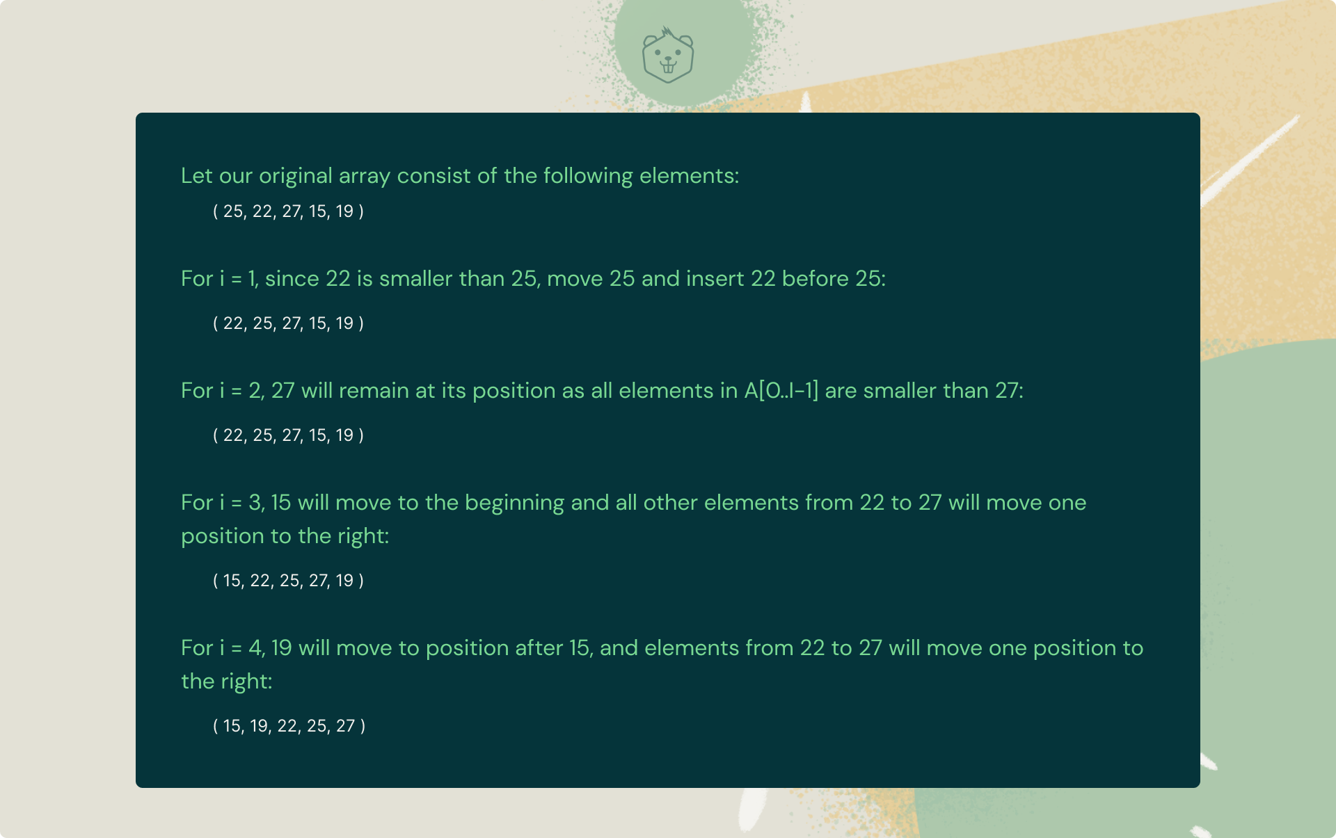
Insertion sort is a sorting algorithm in which the given array is divided into a sorted and an unsorted section. In each iteration, the element to be inserted has to find its optimal position in the sorted subsequence and is then inserted while shifting the remaining elements to the right.
Understanding Insertion Sort algorithm with an example
Here's an example to help you understand insertion sort better:
Now that you've understood how insertion sorting actually works, take a look at its standard C++ implementation.
#include <bits/stdc++.h>
using namespace std;

void Insertion_Sort(int vec[], int n){
	int i, x, j;
	for (i = 1; i < n; i++){
		x = vec[i];
		j = i - 1;
		while (j >= 0 && vec[j] > x){
			vec[j + 1] = vec[j];
			j = j - 1;
		}
		vec[j + 1] = x;
	}
}

int main(){
	int vec[] = { 25, 22, 27, 15, 19 };
	int n = sizeof(vec) / sizeof(vec[0]);
	Insertion_Sort(vec, n);
	for (int i = 0; i < n; i++)
		cout << vec[i] << " ";
	return 0;
}Time Complexity:
- Worst Case: O(n*n)
- Average Case: O(n*logn)
- Best case: O(n*logn)
Auxiliary Space Complexity: O(1)
Use Cases
- This algorithm is stable and is quite fast when the list is nearly sorted.
- It is very efficient when it comes to sorting very small lists (example say 30 elements.)
Try it yourself
Q. Given a list of numbers with an odd number of elements, find the median? [Constraint: Use Insertion Sort]
Input:
- n -> Size of array (n>0)
- 'n' array elements below
Output: A single line representing the required median.
P.S: Don't forget to share your approach with us in the comments below!
4. Quick Sort
Quick Sort is a divide and conquer algorithm. The intuitive idea behind quick sort is it picks an element as the pivot from a given array of elements and then partitions the array around the pivot element. Subsequently, it calls itself recursively and partitions the two subarrays thereafter.
Understanding Quick Sort algorithm with a visualization
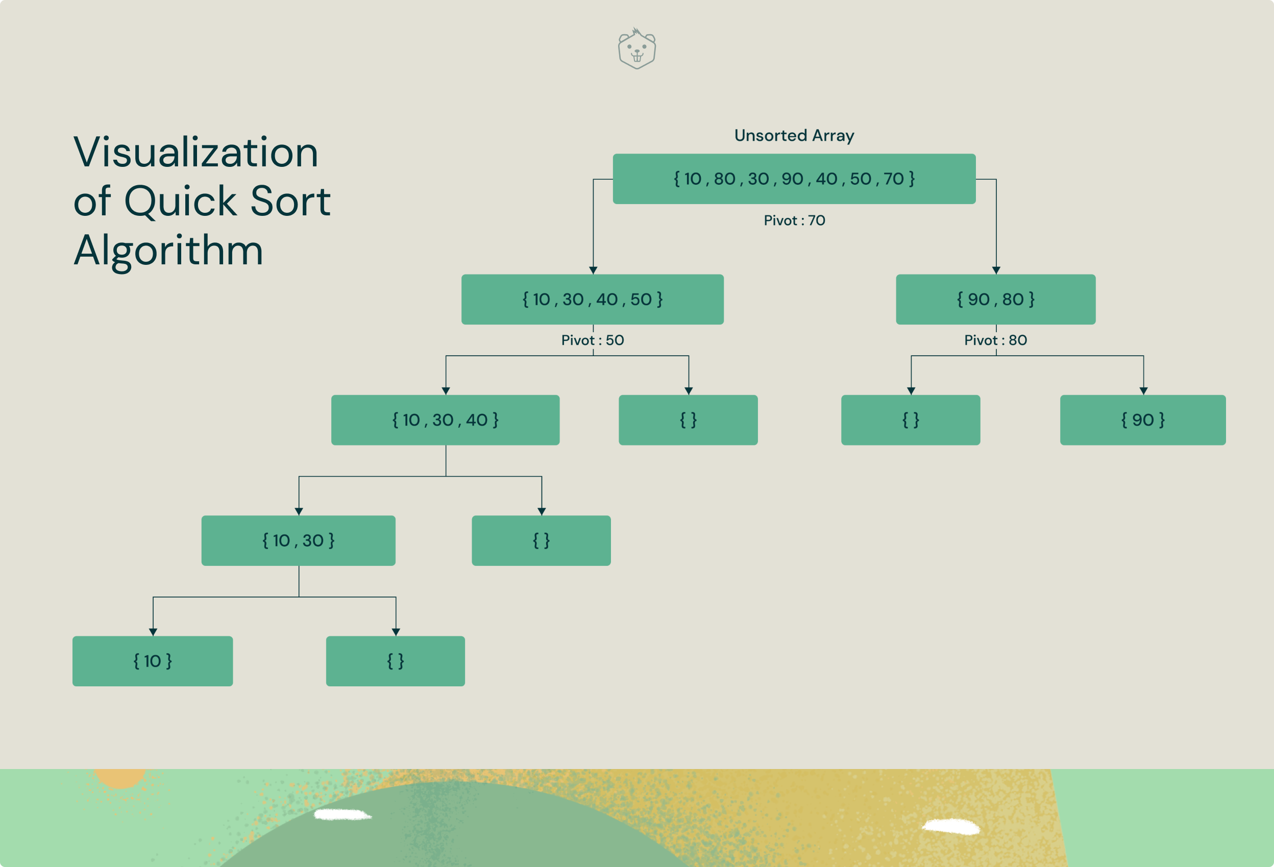
The logical steps involved in Quick Sort algorithm are as follows:
- Pivot selection: Picks an element as the pivot (here, we choose the last element as the pivot)
- Partitioning: The array is partitioned in a fashion such that all elements less than the pivot are in the left subarray while all elements strictly greater than the pivot element are stored in the right subarray.
- Recursive call to Quicksort: Quicksort function is invoked again for the two subarrays created above and steps are repeated.
Comments have been included in the implementation below to help you understand the Quick Sort algorithm better.
#include <bits/stdc++.h>
using namespace std;

int partition (int vec[], int lt, int rt){
	int pivot = vec[rt]; // pivot
	int i = (lt - 1);
	for (int j = lt; j <= rt - 1; j++){
		if (vec[j] < pivot){
			i++; swap(vec[i], vec[j]);
		}
	}
	swap(vec[i + 1], vec[rt]);
	return (i + 1);
}

/* vec[] --> array to be sorted,
lt --> Starting index,
rt --> Ending index*/
void Quick_Sort(int vec[], int lt, int rt){
	if (lt < rt){
		/* mid is partitioning index, vec[p] is now
		at right place */
		int mid = partition(vec, lt, rt);
		// Separately sort elements before
		// partition and after partition
		Quick_Sort(vec, lt, mid - 1);
		Quick_Sort(vec, mid + 1, rt);
	}
}

int main(){
	int vec[] = {14, 21, 5, 2, 3, 19};
	int n = sizeof(vec) / sizeof(vec[0]);
	Quick_Sort(vec, 0, n - 1);
	cout << "Sorted array: ";
	for (int i = 0; i < n; i++)
		cout << vec[i] << " ";
	return 0;
}Time Complexity:
- Worst Case: O(n*n)
- Average Case: O(n*logn)
- Best case: O(n*logn)
Auxiliary Space Complexity: O(1)
Use Cases
- Quick Sort is probably more effective for datasets that fit in memory.
- Quick Sort is appropriate for arrays since is an in-place sorting algorithm (i.e. it doesn’t require any extra storage)
Try it yourself
Q. Given a list of numbers with an odd/even number of elements, find the median? [Constraint: Use Quick Sort]
Input:
- n -> Size of array (n>0)
- 'n' array elements below
Output: A single line representing the required median.
P.S: Need a hint? Drop a comment below.
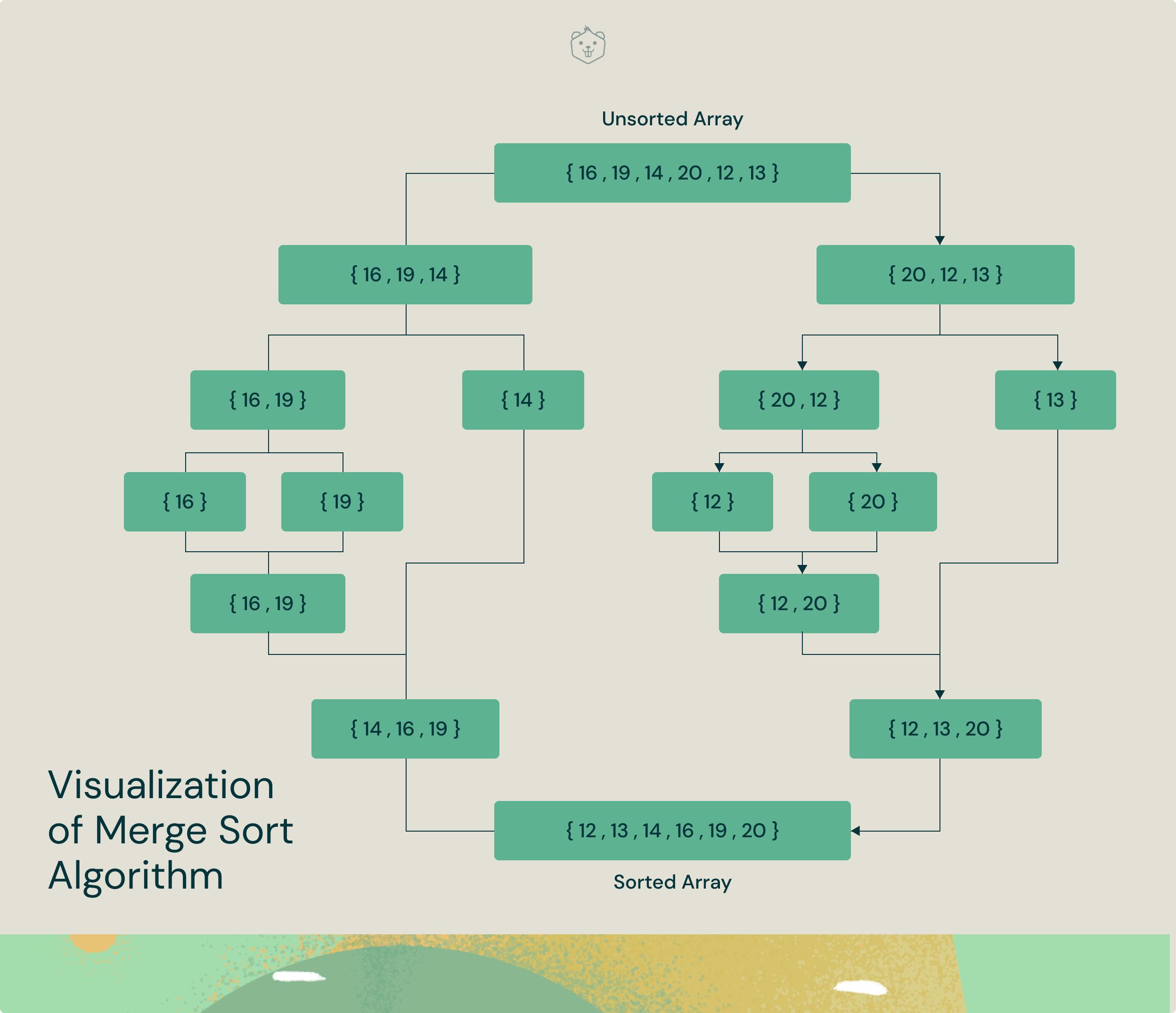
5. Merge Sort
Merge Sort is a divide-and-conquer algorithm. In each iteration, merge sort divides the input array into two equal subarrays, calls itself recursively for the two subarrays, and finally merges the two sorted halves.
Understanding Merge Sort algorithm with a visualization
Now that you're familiar with the intuition behind merge sort, let's take a look at its implementation.
#include <bits/stdc++.h>
using namespace std;

void merge(long vec[], long lt, long m, long rt){
    long n1 = m - lt + 1;
    long n2 = rt - m;
    long L[n1], R[n2];
    for (long i = 0; i < n1; i++)
        L[i] = vec[lt + i];
    for (long j = 0; j < n2; j++) R[j] = vec[m+1+j];
    long i = 0, j = 0;
    long k = lt;
    while (i < n1 and j < n2) {
        if (L[i] <= R[j]) {
            vec[k] = L[i]; i++;
        }
        else {
            vec[k] = R[j]; j++;
        }
        k++;
    }
    while (i < n1) {
        vec[k] = L[i]; i++; k++;
    }
    while (j < n2) {
        vec[k] = R[j]; j++; k++;
    }
}

void Merge_Sort(long vec[],long lt,long rt){
    if(lt>=rt) return;
    long m =lt+ (rt-lt)/2;
    Merge_Sort(vec,lt,m);
    Merge_Sort(vec,m+1,rt);
    merge(vec,lt,m,rt);
}

void printArray(long A[], long size){
    for (long i = 0; i < size; i++)
        cout << A[i] << " ";
}
int main(){
    long arr[] = {16, 19, 14, 20, 12, 13};
    long arr_size = sizeof(arr) / sizeof(arr[0]);
    cout << "Unsorted array is: ";
    printArray(arr, arr_size);
    Merge_Sort(arr, 0, arr_size - 1);
    cout << "\nSorted array is: ";
    printArray(arr, arr_size);
    return 0;
}Time Complexity:
- Worst Case: O(n*logn)
- Average Case: O(n*logn)
- Best case: O(n*logn)
Auxiliary Space Complexity: O(n)
Use Cases
- Merge sort is quite fast in the case of linked lists.
- It is widely used for external sorting where random access can be quite expensive compared to sequential access.
Try it yourself
Q. Find the intersection of two unsorted arrays [Constraint/Hint: Use Merge Sort]
Input:
- n -> Size of array (n>1)
- 'n' array elements below
Output: An array representing the intersection of the two unsorted arrays.
Master Arrays, Linked lists, Stacks/Queues, Trees, and Graphs and build your career (with job guarantee) in Back End or Full Stack development. Here's how.
6. Counting Sort
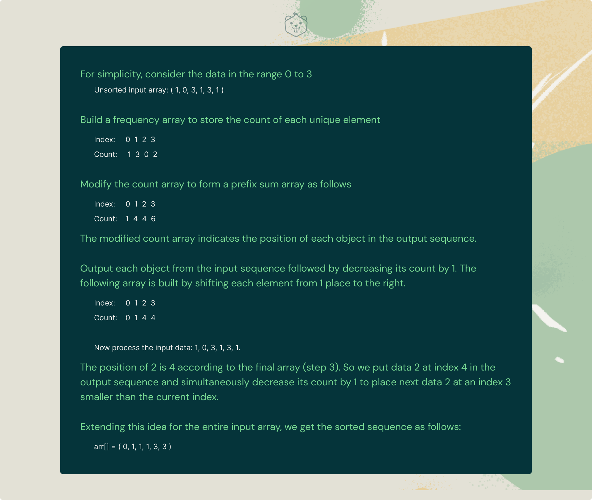
Counting Sort is an interesting sorting technique primarily because it focuses on the frequency of unique elements between a specific range (something along the lines of hashing).
It works by counting the number of elements having distinct key values and then building a sorted array after calculating the position of each unique element in the unsorted sequence.
It stands apart from the algorithms listed above because it literally involves zero comparisons between the input data elements!
Understanding Counting Sort algorithm with an example
Now go ahead and quickly take a look at its implementation in C++
#include<bits/stdc++.h>
using namespace std;

void print(long *vec, long n) {
   for(long i = 1; i<=n; i++)
      cout << vec[i] << " ";
   cout << "\n";
}

long getMax(long vec[], long n) {
   long max = vec[1];
   for(long i = 2; i<=n; i++) {
      if(vec[i] > max)
         max = vec[i];
   }
   return max;
}
void countSort(long *vec, long n) {
   long output[n+1];
   long max = getMax(vec, n);
   long count[max+1];
   for(long i = 0; i<=max; i++)
      count[i] = 0;
   for(long i = 1; i <=n; i++)
      count[vec[i]]++;
   for(long i = 1; i<=max; i++)
      count[i] += count[i-1];
   for(long i = n; i>=1; i--) {
      output[count[vec[i]]] = vec[i];
      count[vec[i]] -= 1;
   }
   for(long i = 1; i<=n; i++) {
      vec[i] = output[i];
   }
}
int main() {
   long n;
   cout << "Enter the size of array: ";
   cin >> n;
   long arr[n+1];
   cout << "Enter elements:" << endl;
   for(long i = 1; i<=n; i++)
      cin >> arr[i];
   cout << "Unsorted array: ";
   print(arr, n);
   countSort(arr, n);
   cout << "Sorted array: ";
   print(arr, n);
}
Time Complexity:
- Worst Case: O(n+k), where n is the size of input array and k is the count of unique elements in the array
Auxiliary Space Complexity: O(n+k)
Use Cases
- Counting sort is quite efficient when it comes to sorting countable objects (such as bounded integers).
- It is also used when sorting is to be achieved in linear complexity.
Try it yourself
Q. Given an array of n input integers, return the absolute difference between the maximum and minimum elements of the array in linear time complexity.
Input:
- n -> Size of array (n>1)
- 'n' array elements below
Output: A single line representing the required difference.
P.S: Don't forget to share your approach with us in the comments below.
Stop scrolling..
You're done with over 50% of the blog. Want to test your knowledge on how well you've understood sorting algorithms so far? Take these quizzes to know where you stand.
Sorting Algorithms Quiz (Level 1)Sorting Algorithms Quiz (Level 2)7. Radix Sort
As you saw earlier, counting sort stands apart because it's not a comparison-based sorting algorithm like Merge Sort or Bubble Sort, thereby reducing its time complexity to linear time.
BUT, counting sort fails if the input array ranges from 1 to n^2 in which case its time complexity increases to O(n^2).
The basic idea behind radix sorting is to extend the functionality of counting sort to get a better time-complexity when input array elements range from 1 till n^2.
Understanding Radix Sort with an example
Algorithm:
For each digit i where i varies from the least significant digit to the most significant digit of a number, sort input array using count sort algorithm according to the ith digit. Remember we use count sort because it is a stable sorting algorithm.
Example:
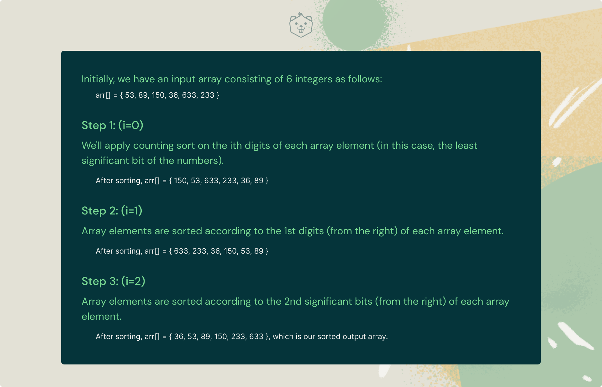
Thus we observe that radix sort utilizes counting sort as its subroutine throughout its execution. Now take a look at its C++ implementation.
#include<bits/stdc++.h>
using namespace std;

long getMax(long vec[], long n){
    long maxval = vec[0];
    for (long i = 1; i < n; i++)
        if (vec[i] > maxval)
            maxval = vec[i];
    return maxval;
}

void Count_Sort(long vec[], long n, long x){
    long res[n];
    long i, count[10] = {0};
    for (i = 0; i < n; i++)
        count[(vec[i] / x) % 10]++;
    for (i = 1; i < 10; i++)
        count[i] += count[i - 1];
    for (i = n - 1; i >= 0; i--) {
        res[count[(vec[i] / x) % 10] - 1] = vec[i];
        count[(vec[i] / x) % 10]--;
    }
    for (i = 0; i < n; i++)
        vec[i] = res[i];
}

void Radix_Sort(long vec[], long n){
    long m = getMax(vec, n);
    for (long x = 1; m / x > 0; x *= 10)
        Count_Sort(vec, n, x);
}

int main(){
    long vec[] = { 53, 89, 150, 36, 633, 233 };
    long n = sizeof(vec) / sizeof(vec[0]);
    Radix_Sort(vec, n);
    for(long i = 0; i < n; i++)
      cout << vec[i] << " ";
    return 0;
}Time Complexity: O(d(n+b)), where b represents the base of array element (eg- 10 represents decimal)
Auxiliary Space Complexity: O(n+d), where d is the maximum number of digits in an array element.
Use Cases
- Radix sorting finds applications in parallel computing.
- It is also used in the DC3 algorithm (Kärkkäinen-Sanders-Burkhardt) while making a suffix array.
Try it yourself:
Q. Given two sorted arrays(arr1[] and arr2[]) of size M and N of distinct elements. Given a value Sum. The problem is to count all pairs from both arrays whose sum is equal to Sum.
Note: The pair has an element from each array. [Constraint: Use Radix Sort]
Input:
- n -> Size of array (n>1)
- 'n' array elements below
Output: A single line representing the required number of pairs
P.S: Don't forget to share your approach with us in the comments below.
8. Bucket Sort
Bucket Sort is a comparison-based sorting technique that operates on array elements by dividing them into multiple buckets recursively and then sorting these buckets individually using a separate sorting algorithm altogether. Finally, the sorted buckets are re-combined to produce the sorted array.
Understanding Bucket Sort algorithm with pseudocode
We can probe further into the working of bucket sort by assuming that we've already created an array of multiple 'buckets' (lists). Elements are now inserted from the unsorted array into these "buckets" based on their properties. These buckets are finally sorted separately using the insertion sort algorithm as explained earlier.
Pseudocode:
Begin
   for i = 0 to size-1
      insert array[i] into the bucket indexed (size * array[i])
   done
   for i = 0 to size-1
      sort bucket[i] using insertion sort
   done
   for i = 0 to size-1
      Combine items of bucket[i] and insert in array in sorted order
   done
End
Well if you're still unsure about the bucket sort algorithm, go back and review the pseudocode one more time.
.
.
Done? All right. Now take a quick look at its implementation below.
#include<bits/stdc++.h>
#define pb push_back
using namespace std;

void Bucket_Sort(float arr[], int n){
	vector<float> bucket[n];
	for (int i = 0; i < n; i++) {
		int bi = n * arr[i];
		bucket[bi].pb(arr[i]);
	}
	for (int i = 0; i < n; i++)
		sort(bucket[i].begin(), bucket[i].end());
	int pos = 0;
	for (int i = 0; i < n; i++)
		for (int j = 0; j < bucket[i].size(); j++)
			arr[pos++] = bucket[i][j];
}

int main(){
	float arr[]= { 0.474, 0.582, 0.452, 0.6194, 0.553, 0.9414 };
	int n = sizeof(arr) / sizeof(arr[0]);
	Bucket_Sort(arr, n);
	cout << "Sorted array is \n";
	for (int i = 0; i < n; i++)
		cout << arr[i] << " ";
	return 0;
}Time Complexity:
- Worst Case: O(n*n)
- Average Case: O(n + k)
- Best case: O(n + k)
Auxiliary Space Complexity: O(k), worst case
Use Cases
- Bucket sorting is used when input is uniformly distributed over a range.
- It is also used for floating point values.
Try it yourself
Q. You are given two arrays, A and B, of equal size N. The task is to find the minimum value of A[0] * B[0] + A[1] * B[1] +…+ A[N-1] * B[N-1], where shuffling of elements of arrays A and B is allowed. [Constraint: Use Bucket Sort]
Input:
- n -> Size of array (n>1)
- 'n' array elements representing the first array
- 'n' array elements representing the second array
Output: A single line representing the required sum
P.S: Need help? Drop a comment below.
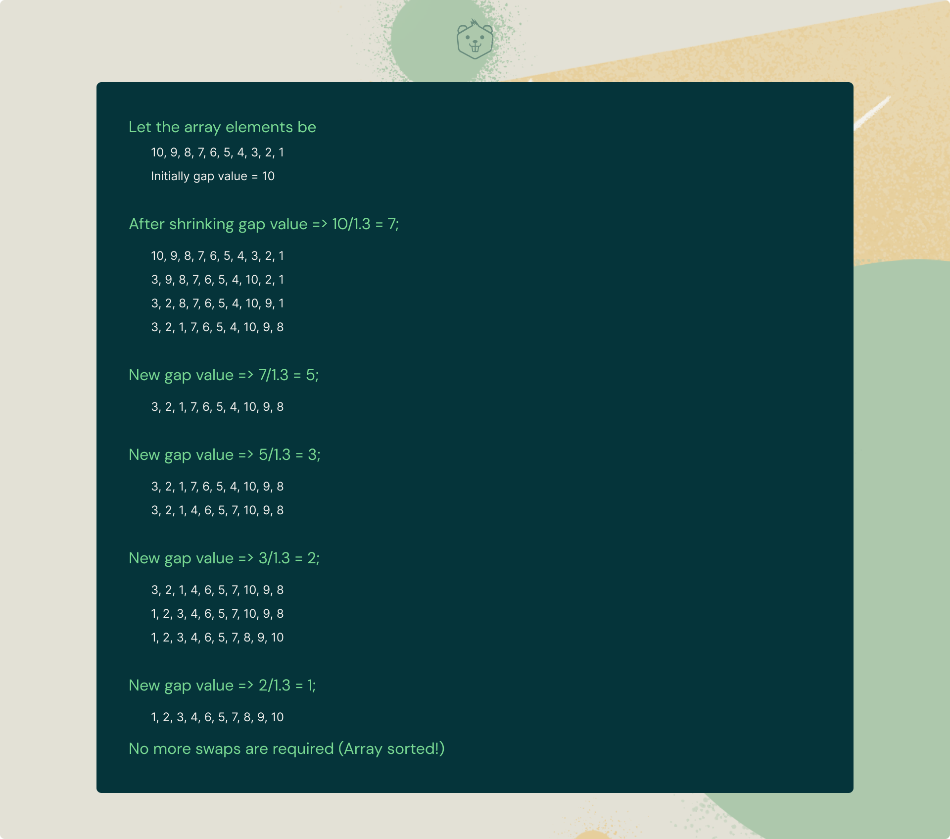
9. Comb Sort
Comb sort is quite interesting. In fact, it is an improvement over the bubble sort algorithm. If you've observed earlier, bubble sort compares adjacent elements for every iteration.
But for comb sort, the items are compared and swapped by a large gap value. The gap value shrinks by a factor of 1.3 for each iteration until the gap value reaches 1, at which point it stops execution.
This shrink factor has been empirically calculated to be 1.3 (after testing Comb Sort algorithm on over 2, 00, 000 random arrays) [Source: Wiki]
Understanding Comb Sort algorithm with a simple example
Pretty simple right? Well, let's have a look at it's C++ implementation:
#include<bits/stdc++.h>
using namespace std;
void Comb_Sort(long *vec, long size) {
   long gap = size;
   bool f = true;
   while(gap != 1 || f == true) {
      gap = (gap)/1.3;
      if(gap<1) gap = 1;
      f = false;
      for(long i = 0; i< size - gap; i++) {
         if(vec[i] > vec[i+gap]) {
            swap(vec[i], vec[i+gap]);
            f = true;
         }
      }
   }
}
int main() {
   long arr[10]={ 10, 9, 8, 7, 6, 5, 4, 3, 2, 1 };
   cout << "Array before Sorting: ";
   for(long i = 0; i < 10; i++)
      cout << arr[i] << " ";
   cout << endl;
   Comb_Sort(arr, 10);
   cout << "Array after Sorting: ";
   for(long i = 0; i < 10; i++)
      cout << arr[i] << " ";
   cout << endl;
}Time Complexity:
- Worst Case: O(n^2)
- Average Case: O(n^2/2^p), where p is a number of increment
- Best case: O(n*logn)
Auxiliary Space Complexity: O(1)
Use Cases
- Comb Sort eliminates small values at the end of the list by using larger gaps.
- It is a significant improvement over Bubble Sort.
Try it yourself
Q. Given an array, find the most frequent element in it. If there are multiple elements that appear maximum number of times, print any one of them. [Constraint: Use Comb Sort]
Input:
- n -> Size of array (n>0)
- 'n' array elements below
Output: A single line representing the element with maximum frequency.
P.S: Did you enjoy this sorting technique? Share your opinions below.
10. Shell Sort
Shell sort algorithm is an improvement over the insertion sort algorithm wherein we resort to diminishing partitions to sort our data.
In each pass, we reduce the gap size to half of its previous value for each pass throughout the array. Thus for each iteration, the array elements are compared by the calculated gap value and swapped (if necessary).
Understanding Shell Sort algorithm with pseudocode
Start
   for gap = N / 2, where gap > 0 and gap updates to gap / 2:
      for i= gap to N – 1:
         for j = j-gap to 0, decrease by gap value:
            if arr[j+gap] >= arr[j]
               break
            else
               swap arr[j+gap] with arr[j]
         done
      done
   done
End
The idea of shell sort is that it permits the exchange of elements located far from each other. In Shell Sort, we make the array N-sorted for a large value of N.
We then keep reducing the value of N until it becomes 1. An array is said to be N-sorted if all subarrays of every N’th element are sorted.
Here, gap size= floor(N/2) for each iteration
Finally, take a look at it's C++ implementation:
#include<bits/stdc++.h>
using namespace std;
int Shell_Sort(int vec[], int n){
	for (int gap = n/2; gap > 0; gap /= 2){
		for (int i = gap; i < n; i ++ ){
			int x = vec[i];
			int j;
			for (j=i; j>=gap && vec[j-gap]>x;j-=gap)
				vec[j] = vec[j - gap];
			vec[j] = x;
		}
	}
	return 0;
}

int main(){
	int vec[] = {10, 9, 8, 7, 6, 5, 4, 3, 2, 1 };
	int n = sizeof(vec)/sizeof(vec[0]), i;
	cout << "Unsorted array: \n";
	for (int i=0; i<n; i++) cout << vec[i] << " ";
	Shell_Sort(vec, n);
	cout << "\nSorted array: \n";
	for (int i=0; i<n; i++) cout << vec[i] << " ";
	return 0;
}Time Complexity:
- Worst Case: Depends on gap size
- Average Case: Depends on gap size
- Best case: O(n*logn)
Auxiliary Space Complexity: O(1)
Use Cases
- Insertion sort does not perform well when the close elements are far apart. Shell sort helps reduce the distance between close elements.
- It is also used when recursion exceeds a limit. The bzip2 compressor compresses it.
Try it yourself
Q. Given an unsorted array of integers. Write a program to remove duplicates from the unsorted array. [Constraint: Use Shell Sort]
Input:
- n -> Size of array (n>1)
- 'n' array elements below
Output: A single line representing the modified array.
Now that you've explored the Top 10 sorting algorithms, all that's left is to answer a few basic questions (just 3 in fact). This will hardly take a minute.
Q1. Which is the best sorting algorithm?
If you've observed, the time complexity of Quicksort is O(n logn) in the best and average case scenarios and O(n^2) in the worst case.
But since it has the upper hand in the average cases for most inputs, Quicksort is generally considered the “fastest” sorting algorithm.
At the end of the day though, the best sorting algorithm comes down to the nature of your input data (and who you ask).
Q2. What is the easiest sorting algorithm?
Bubble sort is widely recognized as the simplest sorting algorithm out there. Its basic idea is to scan through an entire array and compare adjacent elements and swap them (if necessary) until the list is sorted. Pretty simple right?
Q3. Which sorting algorithm would you prefer for nearly sorted lists?
When it comes to sorting nearly sorted data, insertion sort is the clear winner particularly because it's time complexity reduces to O(n) from a whopping O(n^2) on such a sample.
On the other hand, merge sort or quick sort algorithms do not adapt well to nearly sorted data.
Well, that's about it. At the end of the day, it's up to you to decide which sorting technique suits you the best. And yes, don't forget to try out the practice problems served alongside with each sorting technique.
How comfortable are you with sorting now?
Before you go for your next interview, be sure to know the answers to these commonly asked Sorting Algorithms questions. If you read this blog thoroughly, you're all set to get a perfect score. Ready to take the quiz?
Start QuizGo beyond video-based certification courses and online bootcamps. Build the confidence you need to take on Data Structures and Algorithm questions in your next big interview and land your dream job as a Backend Developer or Full Stack Developer - Guaranteed! Find out how.
Additional resources
Don't miss these free learning resources that are an absolute essential for all developers:
- 100+ Essential Linux commands You Must Know. Download PDF >>
- Useful VScode shortcuts To Become A Ninja Programmer. Download PDF >>
- Git commands Cheat Sheet. Download Cheat Sheet >>
- 20+ Interesting Tech Projects with Step-By-Step Instructions. Download Projects >>
Found this article interesting? Show your love by upvoting this article.
We would also love to know the sorting technique that got you excited the most - let us know in the comments below.
Also, if you enjoyed reading this article, don't forget to share it with your friends!